What is a low pass filter? A Guide to the Basics of Passive RC Filters

Time domain and frequency domain

When you look at an electrical signal on an oscilloscope, you see a line that represents changes in voltage versus time. At any given time, the signal has only one voltage value. On an oscilloscope you see a time domain representation of the signal .

A typical waveform is simple and intuitive, but it also has some limitations because it does not directly reveal the frequency content of the signal. Unlike the time domain representation, in which one instant in time corresponds to only one voltage value, the frequency domain representation (also called spectrum ) conveys information about a signal by identifying different frequency components that are presented simultaneously.

Figure 1 – Time domain representations of sine (top) and square wave (bottom) signals

Figure 2 – Frequency representations of sinusoidal (top) and square wave (bottom) signals

▍ General construction algorithm

There are several approaches to designing FIR filters, of which the simplest and most intuitive is the following:

In the frequency domain, the desired frequency response of the filter is set;
The inverse Fourier transform is performed:
A window function is imposed.

It can be performed both purely analytically and numerically using the discrete Fourier transform (hereinafter FFT). The analytical solution is more complex and has the obvious limitation of using only those functions for which Fourier transforms are known.

What is a filter?

A filter is a circuit that removes or “filters out” a specific range of frequency components. In other words, it divides the signal spectrum into frequency components that will be transmitted further , and frequency components that will be blocked .

Unless you have a lot of experience with frequency domain analysis, you may be unsure of what these frequency components are and how they coexist in a signal that cannot have multiple voltage values at the same time. Let's look at a quick example to help clarify this concept.

Let's imagine that we have an audio signal that consists of a perfect 5 kHz sine wave. We know what a sine wave looks like in the time domain, but in the frequency domain we will see nothing but a frequency “spike” at 5 kHz. Now let's assume that we turn on a 500 kHz oscillator, which introduces high-frequency noise into the audio signal.

The signal seen on the oscilloscope will still be just one voltage train with one value at a time, but it will look different because its time domain variations should now reflect both the 5 kHz sine wave and the high frequency oscillations noise.

However, in the frequency domain, the sine wave and noise are separate frequency components that are present simultaneously in that one signal. A sine wave and noise occupy different parts of the frequency domain representation of a signal (as shown in the diagram below), and this means that we can filter out the noise by routing the signal through a circuit that allows low frequencies to pass through and blocks high frequencies.

Figure 3 – Frequency domain representation of audio signal and high-frequency noise

Filter types

Depending on the characteristics of the amplitude-frequency characteristics, filters can be divided into broad categories. If a filter allows low frequencies to pass through and blocks high frequencies, it is called a low pass filter. If it blocks low frequencies and allows high frequencies, it is a high pass filter. There are also bandpass filters, which only pass a relatively narrow range of frequencies, and notch filters, which only block a relatively narrow range of frequencies.

Figure 4 – Amplitude-frequency characteristics of filters

Filters can also be classified according to the types of components that are used to implement the circuit. Passive filters use resistors, capacitors, and inductors; these components are unable to provide gain, and therefore a passive filter can only maintain or reduce the amplitude of the input signal. An active filter, on the other hand, can filter a signal and apply gain because it includes an active component such as a transistor or operational amplifier.

Figure 5 – This active low-pass filter is based on the popular Sallen-Key topology

This article discusses the analysis and design of passive low-pass filters. These circuits play an important role in a wide variety of systems and applications.

RC low pass filter

To create a passive low pass filter, we need to combine a resistive element with a reactive element. In other words, we need a circuit that consists of a resistor and either a capacitor or an inductor. In theory, a resistor-inductor (RL) low-pass filter topology is equivalent, in terms of filtering capacity, to a resistor-capacitor (RC) low-pass filter topology. However, in practice the resistor-capacitor version is much more common, and hence the remainder of this article will focus on the RC low-pass filter.

Figure 6 – RC low pass filter

As you can see in the diagram, the low-pass frequency response of an RC filter is created by placing a resistor in series with the signal path and a capacitor in parallel with the load. In a diagram, the load is a single component, but in a real circuit it could represent something much more complex, such as an analog-to-digital converter, an amplifier, or the input stage of an oscilloscope that you use to measure the frequency response of a filter.

We can intuitively analyze the filtering effect of an RC low-pass filter topology if we understand that the resistor and capacitor form a frequency-dependent voltage divider.

Figure 7 – RC low pass filter redrawn to look like a voltage divider

When the input signal frequency is low, the capacitor impedance will be high relative to the resistor impedance; thus, most of the input voltage drops across the capacitor (and the load that is parallel to the capacitor). When the input frequency is high, the capacitor impedance will be low compared to the resistor impedance, which means more voltage drops across the resistor and less voltage is transferred to the load. Thus, low frequencies are allowed to pass through and high frequencies are blocked.

This qualitative explanation of the operation of an RC low-pass filter is an important first step, but it is not very useful when we need to design an actual circuit because the terms "high frequency" and "low frequency" are extremely vague. Engineers must create circuits that allow and block specific frequencies. For example, in the audio system described above, we want to retain the 5 kHz signal and suppress the 500 kHz signal. This means we need a filter that goes from passing to blocking somewhere between 5 kHz and 500 kHz.

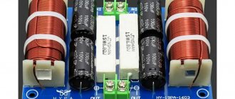
Analysis of the filter from Aliexpress

In order for you to grasp the previous idea, we will analyze a simple example from our narrow-eyed brothers. Aliexpress sells various subwoofer filters. Let's consider one of them.

As you noticed, the filter characteristics are written on it: this type of filter is designed for a 300-watt subwoofer, its characteristic slope is 12 dB/octave. If you connect a subwoofer with a coil resistance of 4 ohms to the filter output, the cutoff frequency will be 150 Hz. If the resistance of the subwoofer coil is 8 ohms, then the cutoff frequency will be 300 Hz.

For full teapots, the seller even provided a diagram in the product description. She looks like this:

Next we assemble this circuit in Proteus. Since when capacitors are connected in parallel, the ratings are summed up, I immediately replaced 4 capacitors with one.

Most often you can see the DC coil resistance value directly on the speakers: 2 Ω, 4 Ω, 8 Ω. Less often 16 Ω. The Ω symbol after the numbers indicates Ohms. Also remember that the coil in the speaker is inductive.

How does an inductor behave at different frequencies?

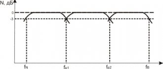
Cutoff frequency

The range of frequencies for which the filter does not cause significant attenuation is called the passband , and the range of frequencies for which the filter causes significant attenuation is called the stopband . Analog filters, such as the RC low-pass filter, always transition from passband to stopband gradually. This means that it is impossible to identify a single frequency at which the filter stops passing signals and begins to block them. However, engineers need a way to conveniently and concisely characterize the frequency response of a filter, and this is where the concept of cutoff frequency .

When you look at the frequency response graph of an RC filter, you will notice that the term “cutoff frequency” is not very accurate. A picture of the spectrum of a signal being "cut" into two halves, one of which is retained and the other discarded, is not applicable because the attenuation increases gradually as frequencies move from values below the cutoff frequency to values above the cutoff frequency.

The cutoff frequency of an RC low-pass filter is actually the frequency at which the amplitude of the input signal is reduced by 3 dB (this value was chosen because a 3 dB reduction in amplitude corresponds to a 50% reduction in power). Thus, the cutoff frequency is also called the -3 dB frequency , and this name is actually more accurate and more descriptive. The term bandwidth refers to the bandwidth of the filter, and in the case of a low-pass filter, the bandwidth is equal to the frequency -3 dB (as shown in the diagram below).

Figure 8 – This diagram shows the general features of the amplitude-frequency response of an RC low-pass filter. The bandwidth is equal to the frequency -3 dB.

As explained above, the low-pass pass behavior of an RC filter is due to the interaction between the frequency-independent impedance of the resistor and the frequency-dependent impedance of the capacitor. To determine the details of a filter's frequency response, we need to mathematically analyze the relationship between resistance (R) and capacitance (C); we can also manipulate these values to design a filter that meets precise specifications. The cutoff frequency (fcf) of the RC low pass filter is calculated as follows:

\[f_{avg} = \frac{1}{2\pi RC}\]

Let's look at a simple example. Capacitor values are more restrictive than resistor values, so we'll start with a common capacitance value (such as 10 nF) and then use a formula to determine the required resistance value. The goal is to design a filter that will preserve the 5 kHz audio signal and reject the 500 kHz noise. We'll try a cutoff frequency of 100 kHz, and later in this article we'll analyze the effect of this filter on both frequency components more closely.

\[100 \times 10^3 = \frac{1}{2 \pi R (10\times 10^{-9})} \\ \Rightarrow R=\frac{1}{2 \pi (10\times 10^{-9})(100 \times 10^3)} = 159.15 \Ohm\]

Thus, a 160 Ohm resistor in combination with a 10 nF capacitor will give us a filter that gives a frequency response close to the required one.

Calculation of the amplitude-frequency response of the filter

We can calculate the theoretical behavior of a low-pass filter using a frequency-dependent version of a typical voltage divider calculation. The output voltage of a resistive voltage divider is expressed as follows:

Figure 9 – Resistive voltage divider

\[V_{out} = V_{in} \left( \frac{R_2}{R_1 + R_2} \right)\]

An RC filter uses an equivalent structure, but instead of R2 we have a capacitor. First we replace R2 (in the numerator) with the reactance of the capacitor (XC). Next we need to calculate the value of the impedance and place it in the denominator. Thus we have

\[V_{out} = V_{in} \left( \frac{X_C}{\sqrt{R_1^2+X_C^2}} \right)\]

The reactance of a capacitor indicates the amount of resistance to the flow of current, but, unlike active resistance, the amount of resistance depends on the frequency of the signal passing through the capacitor. So we have to calculate the reactance at a certain frequency and the formula we use for this is the following:

\[X_C=\frac{1}{2 \pi f C}\]

In the example circuit above, R ≈ 160 ohms, and C = 10 nF. Let's assume that the amplitude of Vin is 1 V, so we can simply remove Vin from the calculations. First, let's calculate the amplitude of Vout at the frequency of the sinusoid we need:

\[X_{C\_5kHz} = \frac{1}{2 \pi (5000)(10 \times 10^{-9})}= 3183\ Ohm\]

\[V_{out\_5kHz} = \frac{3183}{\sqrt{3183^2+160^2}}= 0.999 \V\]

The amplitude of the sinusoidal signal we need practically does not change. This is good since we intended to preserve the sine wave while suppressing noise. This result is not surprising since we chose a cutoff frequency (100 kHz) that is much higher than the frequency of the sine wave (5 kHz).

Now let's see how successfully the filter will attenuate the noise component.

\[X_{C\_500kHz} = \frac{1}{2 \pi (500 \times 10^3)(10 \times 10^{-9})}= 31.8\ Ohm\]

\[V_{out\_500kHz} = \frac{31.8}{\sqrt{31.8^2+160^2}}= 0.195 \V\]

The noise amplitude is only about 20% of the original value.

Visualization of the amplitude-frequency response of the filter

The most convenient way to assess the influence of a filter on a signal is to study the graph of its amplitude-frequency response. These graphs, often called Bode plots, plot amplitude (in decibels) on the vertical axis and frequency on the horizontal axis; the horizontal axis is usually on a logarithmic scale, so the physical distance between 1 Hz and 10 Hz is the same as the physical distance between 10 Hz and 100 Hz, between 100 Hz and 1 kHz, and so on. This configuration allows us to quickly and accurately evaluate the filter's behavior over a very wide frequency range.

Figure 10 – Example of amplitude-frequency response graph

Each point on the curve indicates the amplitude that the output signal would have if the input signal had a magnitude of 1 V and a frequency equal to the corresponding value on the horizontal axis. For example, when the input signal frequency is 1 MHz, the output signal amplitude (assuming the input signal amplitude is 1 V) will be 0.1 V (since –20 dB corresponds to a decrease of ten times).

The general appearance of this frequency response curve will become very familiar as you spend more time with filter circuits. The curve is almost perfectly flat across the passband, and then as the input signal frequency approaches the cutoff frequency, the rate of its rolloff begins to increase. Eventually, the rate of change of attenuation, called roll-off, stabilizes at 20 dB/decade, that is, the output signal level decreases by 20 dB for every tenfold increase in the input signal frequency.

Evaluating Low Pass Filter Performance

If we plot the amplitude-frequency response of the filter we designed earlier in this article, we see that the amplitude response at 5 kHz is essentially 0 dB (i.e., almost zero attenuation), and the amplitude response at 500 kHz is approximately –14 dB (corresponding to a gain of 0.2). These values are consistent with the results of the calculations we performed in the previous section.

Since RC filters always have a smooth transition from passband to stopband, and the attenuation never reaches infinity, we cannot design a "perfect" filter, that is, a filter that does not affect the desired sine wave signal and completely eliminates noise. Instead, we always have a compromise. If we move the cutoff frequency closer to 5 kHz, we get more attenuation of the noise, but also more attenuation of the useful sine wave signal we want to send to the speaker. If we move the cutoff frequency closer to 500 kHz, we get less attenuation at the desired signal frequency, but also less attenuation at the noise frequency.

Autotransformer and transformer connection

If you want to get a sharper resonant curve, you can use a transformer (Fig. 3) or autotransformer (Fig. 4) connection to supply the input voltage.

Rice. 3. Transformer connection.

Rice. 4. Autotransformer connection.

The number of turns of the coupling coil (Fig. 3) or the number of tap turns (counting from the grounded end of the coil) can be determined from the formula: R1 = Ro(N/No)^2, where R1 is actually the output resistance of the input alternating voltage source, Ro is the resistance of the circuit at the resonant frequency, N is the number of turns of the coupling coil (or the number of turns from which the tap is made), No is the number of turns of the circuit coil (or the total number of turns of the coil, if according to Fig. 4).

Rice. 5. Capacitive autotransformer.

It is not at all necessary to make a tap specifically from the coil; you can also make a tap from the capacitor, or rather from the capacitive component of the circuit. So it turns out - a capacitive autotransformer (Fig. 5).

And the ratio of capacitances for a certain value of the output resistance of the signal source can be determined from the formula: R1 = Ro * C1^2 / (C1+C2)^2.

The circuit can be influenced by shunting not only by the output resistance of the source Uin, but also by the input resistance of the cascade, which receives the output voltage Uout from the circuit (R2 in Fig. 6). Especially if the input resistance of the cascade (R2) is small (comparable or even less than Ro).

Rice. 6. Filter circuit.

In this case, it is necessary to first calculate the new value of Ro, reduced by parallel connection of resistance R2. The calculation is made using the well-known parallel resistance formula:

R = (RoR1) / (Ro+R2).

And then calculate the agreement (taking the resulting value of R as Ro in the formulas).

Low Pass Filter Phase Shift

So far we have discussed the way a filter changes the amplitude of various frequency components in a signal. However, reactive circuit elements always introduce a phase shift in addition to influencing amplitude.

The concept of phase refers to the value of a periodic signal at a certain point in the cycle. Thus, when we say that a circuit causes a phase shift, we mean that it creates an offset between the input and output signals: the input and output signals no longer begin and end their cycles at the same point in time. The phase shift value, such as 45° or 90°, indicates how much offset was created.

Each reactive element in the circuit introduces a 90° phase shift, but this phase shift does not occur immediately. The phase of the output signal, as well as the amplitude of the output signal, changes gradually as the frequency of the input signal increases. In an RC low pass filter, we have one reactive element (capacitor) and hence the circuit will eventually introduce a 90° phase shift.

As with amplitude-frequency response, phase-frequency response is most easily assessed by examining a graph in which the frequency on the horizontal axis is plotted on a logarithmic scale. The description below gives a general idea and then you can fill in the details by looking at the chart.

The phase shift is initially 0°.
It gradually increases until it reaches 45° at the cutoff frequency; in this section of the characteristic the rate of change increases.
After the cutoff frequency, the phase shift continues to increase, but the rate of change decreases.
The rate of change becomes very small as the phase shift asymptotically approaches 90°.

Figure 11 - The solid line is the amplitude-frequency characteristic, and the dotted line is the phase-frequency characteristic. The cutoff frequency is 100 kHz. Note that at the cutoff frequency the phase shift is 45°.

Second order low pass filters

So far we have assumed that an RC low pass filter consists of one resistor and one capacitor. This configuration is a first order filter .

The "order" of a passive filter is determined by the number of reactive elements, that is, capacitors or inductors, that are present in the circuit. A higher order filter has more reactive elements, which results in a larger phase shift and a steeper frequency response rolloff. This second characteristic is the main reason for increasing the filter order.

By adding one reactive element to the filter, for example going from first to second order or from second to third order, we increase the maximum roll-off by 20 dB/decade. A steeper roll-off results in a faster transition from low attenuation to high attenuation, and this can lead to improved performance when there is no wide bandwidth separating the necessary frequency components from the noise components.

Second-order filters are usually built around a resonant circuit consisting of an inductor and a capacitor (this topology is called "RLC", i.e. resistor-inductor-capacitor). However, it is also possible to create second-order RC filters. As shown in the figure below, all we need to do is cascade two first order RC filters.

Figure 12 – Second order RC low pass filter

While this topology certainly produces a second-order response, it is not widely used—as we will see in the next section, its frequency response is often inferior to that of a second-order active filter or a second-order RLC filter.

Simplified formulas

For simple calculation of filters, the following are simplified formulas borrowed from an engineering reference book.

The formulas contain a coefficient of 160000 (one hundred and sixty thousand). This figure arises for two reasons.

Firstly, it is assumed to take the capacitance value in microfarads (10-6 Farads)
Secondly, when moving from a circular frequency to a cyclic one, a factor of 2π appears

Respectively:

1 / (2⋅π⋅10-6) = 159154 ≈ 160000

So, let's move on to the filters themselves.

Amplitude-frequency response of a second-order RC filter

We can try to create a second order RC low pass filter by designing the first order filter according to the required cutoff frequency and then connecting these two first order stages in series. This will produce a filter that has a similar overall frequency response and a maximum roll-off of 40 dB/decade instead of 20 dB/decade.

However, if we look at the frequency response more closely, we will see that the frequency has decreased by -3 dB. The second order RC filter does not behave as expected because the two links are not independent - we cannot simply connect the two links together and analyze the circuit as a first order low pass filter followed by an identical first order low pass filter.

Moreover, even if we insert a buffer between these two links so that the first RC link and the second RC link can act as independent filters, the attenuation at the original cutoff frequency will be 6 dB instead of 3 dB. This is precisely because the two stages operate independently - the first filter introduces 3 dB of attenuation at the cutoff frequency, and the second filter adds another 3 dB of attenuation.

Figure 13 – Comparison of amplitude-frequency characteristics of second-order low-pass filters

The main limitation of a second-order RC low-pass filter is that the designer cannot fine-tune the transition from passband to stopband by adjusting the quality factor (Q) of the filter; This parameter indicates how smooth the amplitude-frequency response is. If you cascade two identical RC low pass filters, the overall transfer function is the same as the second order response, but the quality factor is always 0.5. When Q = 0.5, the filter is on the verge of excessive attenuation, and this results in a frequency response that sags in the transition region. Second-order active filters and second-order resonant filters do not have this limitation; the designer can control the quality factor and thus fine-tune the amplitude-frequency response in the transition region.

Calculation of passive crossover filters in acoustic systems

This article will help you calculate electrical filters. The calculation accuracy is high, but still, to accurately adjust the frequency response, it is necessary to use a microphone, since here the frequency response and impedance are conventionally considered ideal.

Crossover filters with a flat frequency response have a number of advantages over other types of filters, and are currently the most used in HI-FI class speakers. Therefore, only this type of filter will be considered in the calculation methodology. The essence of the calculation is that the isolation filters are first calculated from the condition of an active load and a voltage source with an infinitesimal output resistance (which is true for modern audio amplifiers). Then measures are taken to reduce the influence of amplitude-frequency and phase-frequency distortions of loudspeakers and the complex nature of their input impedance on the characteristics of the filters.

The calculation of crossover filters begins with determining their order and finding the parameters of the elements of the prototype low-pass ladder filter.

A prototype filter is a low-pass ladder filter, the values of which elements are normalized relative to a unit cutoff frequency and a unit active load. Having calculated the elements of a low-pass filter of a certain order at a real frequency and a real value of load resistance, it is possible, by applying frequency conversion, to determine the circuit and calculate the values of the elements of a high-pass filter and a band-pass filter of the corresponding order. The normalized values of the elements of a prototype filter operating from a voltage source are determined by expanding its output conductivity into a continued fraction. The normalized values of prototype filter elements for calculating “all-pass type with flat frequency response” separation filters of the 1st...6th order are summarized in the table:

Filter order	The value of the normalized z value parameters
Filter order	1	2	3	4	5	6
1	1,0	–	–	–	–	–
2	2,0	0,5	–	–	–	–
3	1,5	1,33	0,5	–	–	–
4	1,88	1,59	0,94	0,35	–	–
5	1,54	1,69	1,38	0,89	0,31	–
6	1,8	1,85	1,47	1,12	0,73	0,5

Figure 1 shows a diagram of a sixth-order prototype filter. Prototype filter circuits of lower orders are formed by discarding the corresponding elements - α (starting with the largest ones) - for example, a 1st order prototype filter consists of one inductance α1 and a load R n .

Rice. 1. Circuit diagram of a one-way loaded prototype low-pass filter of the 6th order

The value of the real parameters of the elements corresponding to the selected order of the isolation filters, the load resistance R n (Ohm) and the cutoff (separation) frequency f d (Hz) are calculated as follows:

a) for a low-pass filter:

each element α-inductance of the prototype filter is converted into real inductance (H), calculated by the formula:

L=αR n / 2πf d [1]

each element α -capacitance of the prototype filter is converted into real capacitance (F), calculated by the formula:

C=α/ 2πf d R n [2]

b) for a high pass filter:

each element α -inductance of the prototype filter is replaced by real capacitance calculated by the formula:

C= 1/2πf d αR n [3]

each element α -capacitance of the prototype filter is replaced by real inductance, calculated by the formula:

L=R n / 2πf d α [4]

c) for a bandpass filter:

each α -inductance is replaced by a series circuit consisting of real L and C -elements, calculated using the formulas

L=αR n / 2π(f d 2 -f d 1 ) [5]

where f d 2 and f d 1 are the lower and upper cutoff frequencies of the bandpass filter, respectively,

С= 1/4π2f02L [6]

where f0=√ f d 1 f d 2 – average frequency of the bandpass filter.

Each α-capacitance element is replaced by a parallel circuit consisting of real L and C-elements, calculated using the formulas:

C=α/ 2π(f d 2 -f d 1 )R n , [7]

L= 1/4π2f02C [8]

Example. It is required to calculate the values of the elements of separate filters for a three-way speaker system.

We select second-order separation filters. Let the selected values of the separation frequencies be: between the low-frequency and mid-frequency channels f d 1 =500 Hz, between mid-frequency and high-frequency f d 2 =5000 Hz. DC speaker impedance: low-frequency and mid-frequency – 8 Ohms, high-frequency – 16 Ohms.

Rice. 2. An example of calculating crossover filters for a three-way speaker : a) frequency response of loudspeakers without filters; b) frequency response of loudspeakers with filters, matching and correction circuits; c) total frequency response of the speakers on the working axis and when the microphone is displaced by an angle of ±10° in the vertical plane

The amplitude-frequency characteristics of the loudspeakers, measured in an anechoic chamber on the working axis of the speaker at a distance of 1 m, are shown in Fig. 2, a) (low-frequency loudspeaker 100GD-1 , mid-frequency 30GD-8 , high-frequency 10GD-43 ).

Let's calculate the low pass filter:

The value of the normalized parameters of the elements is determined from the table: α1 = 2.0, α2 =0.5.

From Fig. 1 we determine the circuit of the prototype low-pass filter: the filter consists of inductance α1 , capacitance α2 and load Rн .

The values of real elements of low-pass filters are found using expressions [1] and [2]:

L 1 LF =αR n / 2πf d 1 =2.0 8.0/(2 3.14 500) = 5.1 mH,

C 1 LF =α/ 2πf d 1 R n =0.5/(2·3.14·500·8.0)=20 µF.

The values of the bandpass filter elements (for a mid-frequency loudspeaker) are determined in accordance with the expressions [5]…[8]:

L 1 MF =α 1 Rн/2π(f d 2 -f d 1 )=2.0 8.0/2 3.14(5000-500)=0.566 mH (HF side)

With 1 midrange = 1/4π2f02L1 midrange = 1/4 3.142 5000 500 5.66 10-4 = 18 µF (low frequency side)

C 2 MF =α 2 / 2π(f d 2 -f d 1 )R n =0.5/2 3.14(5000-500) 8.0 = 2.2 μF (HF side)

L 2 MF = 1/4π2f02C2 MF = 1/4 3.142 5000 500 2.2 10-6 = 4.6 mH (LF side)

The values of the high-pass filter elements are determined in accordance with expressions [3] and [4]:

C 1 HF = 1/2πf d 2 α 1 R n =1/(2·3.14·5000·2.0·16)=1.00 µF,

L 2 HF =R n / 2πf d 2 α 2 =16/(2·3.14·5000·2.0)=0.25 mH.

To match the filters with the input impedance of the loudspeakers, a special matching circuit can be used. In the absence of this circuit, the input impedance of the loudspeaker affects the frequency response and phase response of the crossover filters. The parameters of the elements of the matching circuit connected in parallel with the loudspeaker are found from the condition:

Y c ( s )+ Y GR ( s )=1/ R E ,

where Y c ( s ) is the conductivity of the matching circuit, Y GR ( s ) is the input conductivity of the loudspeaker, R E is the electrical resistance of the loudspeaker at direct current.

The matching circuit diagram is shown in Fig. 3. The circuit is dual to the equivalent loudspeaker circuit. The values of the circuit elements are determined as follows:

R K 1 = R E , [9]

C K 1 = L VC / R E 2 [10]

R K = RE2/RES=QESRE/QMS,

C K =LCES/ RE2=1/QESRE2 π f s ,

L K =CMES R E 2 =QESRE/2 π f s ,

where L VC is the inductance of the voice coil, f s , C MES , L CES , R ES are the electromechanical parameters of the loudspeaker.

To compensate for the input impedance of a low-frequency loudspeaker, a simplified circuit is used, consisting of resistance RK1 and capacitance CK1 . This is because the mechanical resonance of the loudspeaker does not affect the low-pass filter characteristics and only compensates for the inductive nature of the loudspeaker input impedance. It is advisable to connect a complete matching network to high-frequency and mid-range loudspeakers if the resonant frequency of the loudspeaker is near the cutoff frequency of the high-pass filter or the low cutoff frequency of the bandpass filter. In the event that the cutoff frequencies of the filters are significantly higher than the resonant frequencies of the loudspeakers, the inclusion of a simplified circuit is sufficient.

Fig.3 . Matching circuit diagram to compensate for the complex nature of the loudspeaker input impedance

The influence of the input complex impedance of loudspeakers can be considered using the example of second-order separation filters of high and low frequencies [3] (Fig. 4).

Rice. 4. Electrical equivalent circuit of a loudspeaker with 2nd order crossover filters: a – with a low-pass filter; b – with a high-pass filter; (1 – filter; 2 – loudspeaker)

The parameters of the low-frequency loudspeaker are selected in such a way that its frequency response corresponds to the Butterworth approximation, i.e. total quality factor Q ts =0.707. The cutoff frequency of the low-pass filter is chosen to be 10 times greater than the resonant frequency of the loudspeaker fd=10fs . The voice coil inductance is selected from the condition: QVC = 0.1, where QVC is the quality factor of the voice coil, defined as:

Q VC =LVC2π f s / R E ,

where fs is the resonant frequency of the loudspeaker, RE is the DC resistance of the voice coil, LVC is the inductance of the voice coil.

The value QVC =0.1 corresponds to the average value of the voice coil inductance of powerful low-frequency loudspeakers. As a result, we can assume that the inductance of the voice coil LVC and the active resistance R E are connected in parallel with the filter capacitance C1 and form a wide maximum in the frequency response of the input impedance in the region of the filter cutoff frequency, followed by a sharp dip (Fig. 5, a). The corresponding changes in the frequency response of the voltage filter consist of a slight rise in the frequency response at frequency f ≈ 2 f s (due to the inductance of the voice coil) and a smooth dip, followed by a sharp peak in the frequency response due to the resonance of the circuit formed by the inductance of the voice coil and the capacitance of the crossover filter. The corresponding changes in the frequency response and ZBX after switching on a matching circuit consisting of a series-connected resistor and capacitor are shown in Fig. 5a (curves 2, 4, 6). The inclusion of a matching circuit brings the nature of the input impedance of the loudspeaker closer to the active one and the frequency response of the isolation filter in voltage to the desired one. However, due to the influence of the voice coil inductance, the frequency response in terms of sound pressure differs from the desired one (curve 4), therefore, even after the matching circuit, a slight adjustment of the filter elements and the matching circuit is sometimes required.

Rice. 5 Frequency response and input impedance of 2nd order crossover filters loaded onto a loudspeaker: a) low-pass filter; b) high pass filter;

Voltage frequency response at the filter output without a matching circuit;
Voltage frequency response at the output of the filter with a matching circuit;
Frequency response for sound pressure without a matching circuit;
Frequency response for sound pressure with a matching circuit;
input impedance of a filter with a loudspeaker without a matching circuit;
input impedance of a filter with a loudspeaker with a matching network.

In the case of a high-pass filter, the influence of the complex nature of the input impedance of the loudspeaker on the input impedance and frequency response of the filter is of a different nature. If the high-pass filter's cutoff frequency is near the loudspeaker's resonance frequency f s (a case sometimes encountered in mid-range loudspeaker filters, but practically impossible for high-frequency loudspeakers), the input impedance of the high-pass filter with a loudspeaker without a matching network may have a deep dip due to at the loudspeaker resonance frequency f s, its input impedance increases significantly and is purely active. The filter appears to be idling, due to a sharp increase in load resistance, and its input resistance is determined by the series-connected elements C1, L 1 . A more common situation is when the cutoff frequency of the high-pass filter fd is significantly higher than the resonance frequency of the loudspeaker fs . Figure 5b shows an example of the influence of the input impedance of a loudspeaker and its compensation on the frequency response of a high-pass filter in terms of voltage and sound pressure. The filter cutoff frequency is chosen significantly higher than the resonance frequency of the loudspeaker f d ≈8 f s , loudspeaker parameters Q TS = 1.5 , Q MS = 10, QVC = 0.08. A rise in the frequency response in sound pressure and voltage in the high-frequency region, accompanied by a drop in input impedance, is explained by the influence of the inductance of the LVC . At higher frequencies, the frequency response drops, and the input impedance increases due to an increase in the inductive reactance of the voice coil.

Curves 2, 4, 6 in Fig. 5b show the influence of the RC matching circuit.

The output impedance of the high-pass crossover filter, which increases with decreasing frequency, affects the electrical quality factor of the loudspeaker, increasing it, and accordingly increases the total quality factor and the shape of the frequency response in terms of sound pressure. In other words, there is an effect of “dedamping” of the loudspeaker. To achieve this, it is necessary to select the slope of the filter’s frequency response and the cutoff frequency of the high-pass filter f d >> f s so that at the resonance frequency f s the signal attenuation is at least 20 dB.

When calculating the isolation filters in the example discussed above, it was assumed that the nature of the load is active, so we will calculate the matching circuits that compensate for the complex nature of the input impedance of the loudspeaker.

The crossover frequency of the low-frequency and mid-frequency channels f d 1 is selected approximately two octaves higher than the resonant frequency of the mid-frequency loudspeaker, and the crossover frequency of the mid-frequency and high-frequency channels f d 2 is two octaves higher than the resonant frequency of the high-frequency loudspeaker. In addition, it can be assumed that the inductance of the voice coil of a high-frequency loudspeaker is negligible in the operating frequency range and can be ignored (this is true for most high-frequency loudspeakers). In this case, you can limit yourself to using a simplified matching circuit for low-frequency and mid-frequency loudspeakers.

Example. Measured (or determined from the frequency response curve of the input impedance) inductance of the voice coils: low-frequency loudspeaker L VC =3·10-3Г=3 mH , mid-frequency loudspeaker LVC=0.5·10-3 Г=0,5 mH . Then the value of the elements of the compensating circuits is calculated using formulas [9] and [10]:

for low frequency: R K 1 – R π =8 Ohm; SK1=LVC/R2E=3 10-3/64=47 µF

for midrange: R' K 1 = R E -8 Ohm; C'K1=LVC/R2E=0.5 ·10-3/64=8.0 µF.

There is a peak in the frequency response of a mid-frequency loudspeaker, which increases the unevenness of the total frequency response of the speaker (Fig. 2a); in this case, it is advisable to turn on the amplitude corrector. The reduction link (Fig. 6) is used to correct the peaks in the frequency response of loudspeakers or the entire speaker system. This link has a purely active input impedance equal to the load resistance RH and can therefore be connected between a filter and a loudspeaker with compensated input impedance. In the case of turning on the rejecting link at the input of the AC, the circuit can be simplified, since there is no need for elements C q , L q , R q , which ensure the active nature of the input resistance of the link. The values of the elements are calculated using the formulas:

R K ≈ R H (10-0.05 N -1),

L K = R K ∆ f /2π f 0 2 ,

CK=1/LK4π2 f 0 2 ,

C q = L K / R H 2 ,

L q = C K R H 2 ,

Rq = RH ( 1+ RH / RK ) , _ _

where R H is the loudspeaker resistance (compensated) or the input resistance of the speaker (Ohm) in the region of the resonant frequency of the rejector section;

∆ f – frequency band of the adjusted frequency response peak (measured by level – 3 dB), Hz;

f 0 – resonant frequency of the notch, Hz;

N – frequency response peak value, dB.

Rice. 6. Reducing link: a) schematic diagram; b) frequency response

Let's use a rejection link connected between the filter and the mid-frequency loudspeaker with a matching circuit.

From the frequency response of the mid-frequency loudspeaker we determine ∆ f =1850 Hz, f 0 =4000 Hz, N =6 dB. The resistance of the mid-frequency loudspeaker with the matching circuit is R H = 8 Ohms.

The values of the elements of the control link are as follows:

R K ≈ R H (10-0.05 N -1)=8(10-0.05 6-1)=7.96 Ohm,

L K = R K ∆ f /2π f 0 2 =7.96·1850/2π(4000)2=0.147 mH,

C K =1/LK4π2 f 0 2 =1/1.47·10-4(2π4000)2=11 µF,

C q = L K / R H 2 =1.47·10-4/64=2.3 µF,

L q = C K R H 2 =10.8 10-6 64 = 0.7 mH,

R q = R H (1+ R H / R K )=8(1+8/7.96)≈16.0 Ohm.

In the example under consideration, the frequency response of the high-frequency and mid-frequency loudspeaker have average levels approximately 6 dB and, accordingly, 3 dB higher than the frequency response of the low-frequency loudspeaker (the sound pressure was recorded when all speakers were supplied with a sinusoidal voltage of the same magnitude). In this case, to reduce the unevenness of the total frequency response of the speaker, it is necessary to weaken the level of mid-frequency and high-frequency components. This can be done either using a first-order corrective high-frequency link (Fig. 7), the elements of which are calculated using the formulas:

R K ≈ R H (10-0.05 N -1),

L K = R K /2π f d √( 100.1 N -2), N≥3 dB,

Or using L-shaped passive attenuators that provide a given attenuation level N (dB) and a given input impedance RBX (Fig. 8). The value of the attenuator elements is calculated using the formulas:

R 1 ≈ R BX (1-10-0.05 N ),

R 2 ≈ R H R BX 10-0.05 N /( R H – R BX 10-0.05 N ).

Rice. 7. 1st order link, correcting high frequencies: a) circuit diagram; b) frequency response

Rice. 8. Passive L-shaped attenuator

As an example, let us calculate the values of the attenuator elements to attenuate a high-frequency loudspeaker signal by 6 dB. Let the input impedance of the loudspeaker with the attenuator turned on be equal to the input impedance of the loudspeaker, i.e. 16 Ohm, then:

R 1 ≈16(1-10-0.05·6)≈8.0 Ohm, R 2 ≈16·10-0.05·6/(1-10-0.05·6)≈16.0 Ohm .

Similarly, we calculate the values of the attenuator elements for a mid-frequency loudspeaker: R1 = 4.7 Ohms, R 2 = 39 Ohms. Attenuators are switched on immediately after the loudspeakers with matching circuits.

The complete circuit of the isolation filters is shown in Fig. 9, the frequency response of the speaker with the calculated filters is shown in Fig. 2, c.

As mentioned above, even-order filters allow only one option for the polarity of loudspeaker switching; in particular, second-order filters require switching in antiphase. For the example under consideration, the low-frequency and high-frequency loudspeakers must have identical switching polarities, and the mid-frequency loudspeaker must have the opposite polarity. The requirements for the polarity of loudspeakers were discussed above on a speaker model with ideal loudspeakers. Therefore, when turning on real loudspeakers that have their own phase response ≠0 (in the case of choosing crossover frequencies near the boundary frequencies of the operating range of the loudspeakers or when the frequency response of the loudspeakers is highly uneven), the condition for matching the real phase response of the channels may not be met. Therefore, to monitor the real phase response from the sound pressure of loudspeakers with filters, it is necessary to use a phase meter with a delay line or determine the matching condition indirectly by the nature of the total frequency response of the speakers in the channel separation bands. The correct polarity for switching on the loudspeakers can be considered the one that corresponds to less unevenness of the total frequency response in the channel separation band. Accurate matching of the phase response of the separated channels while satisfying all other requirements (flat frequency response, etc.) is carried out using numerical methods for synthesizing optimal separation filters-correctors on a computer.

Fig.9. Schematic diagram of the speaker with calculated isolation filters (capacitance in microfarads, inductance in millihenries, resistance in ohms).

In the development of passive isolation filters, an important role is played by their design, as well as the choice of the type of specific elements - capacitors, inductors, resistors, in particular, the relative placement of the inductors has a great influence on the characteristics of speakers with filters; if they are poorly positioned due to mutual coupling, interference is possible signal between closely spaced coils. For this reason, it is recommended to place them mutually perpendicular; only such an arrangement can minimize their influence on each other. Inductors are one of the most important components of passive coupling filters. Currently, many foreign companies use inductors with cores made of magnetic materials, which provide a large dynamic range, a low level of nonlinear distortion and small dimensions of the coils. However, the design of coils with magnetic cores involves the use of special materials, so until now many developers use coils with air cores, the main disadvantages of which are large dimensions with low losses (especially in the low-frequency channel filter), as well as high copper consumption; advantages - negligible nonlinear distortions.

The air-core inductor configuration shown in Fig. 10 is optimal since it provides the maximum L/R , i.e. a coil with a given inductance L , wound with a wire of a selected diameter, has, for a given winding configuration, the lowest resistance R or the highest quality factor compared to any other. The ratio L/R , which has the dimension of time, is related to the dimensions of the coil by the ratio [3.13]:

L /R=161.7alc/(6a+9l+10c);

L – in microhenry, R – in ohms, a, l, c – in millimeters.

Fig. 10. Inductor coil with an air core of optimal configuration: a) in section; b) appearance.

Calculation ratios for this coil configuration: a=1.5c , l=c ; coil design parameter c=√(L/R8.66) , number of turns N=19.88√( L / c ), wire diameter in millimeters, d=0.841c/√ N , wire weight (material - copper) in grams , q = c 3 /21, wire length in millimeters, B=187.3√ Lc . If the inductor is calculated based on a wire of a given diameter, the main calculation ratios are as follows:

design parameter c =5√( d 4 19.882 L /0.8414)=3.85√(d 4 L ) , wire resistance R=L/ c28.66 .

Let us find, for example, the parameters of the inductor of the previously calculated low-pass filter. The inductance of the coil is L1LF = 5.1 mH . We determine the DC coil resistance R Let the signal attenuation due to losses R in the coil be N≤1dB . Since the DC resistance of the subwoofer is RE =8 Ohms, the permissible coil resistance, determined from the expression R≤RE(100.05N-1), is R≤0.980 Ohms ; then the design parameter of the coil is c =√5100/0.98·8.66=24.5 mm ; number of turns N=19.8√(5100/24.5)=287 turns ; wire diameter d=0.841·24.5/√287=1.2 mm ; wire mass q =24.53/21.4≈697 g ; wire length B =187.3√(85.1·24.5)≈46 m.

Another important element of passive coupling filters are capacitors. Typically, paper or film capacitors are used in filters. The most commonly used paper capacitors are domestic MBGO capacitors. The advantage of these types of capacitors is low losses, high temperature stability, the disadvantage is large dimensions, a decrease in the permissible maximum voltage at high frequencies. Currently, the filters of a number of foreign speakers use electrolytic non-polar capacitors with low internal losses, combining the advantages of the capacitors considered and free from their disadvantages.

Based on materials from the book: “High-quality acoustic systems and radiators”

(Aldoshina I.A., Voishvillo A.G.)

Summary

All electrical signals contain a mixture of desired frequency components and unwanted frequency components. Unwanted frequency components are typically caused by noise and interference, and in some situations they will negatively impact system performance.
A filter is a circuit that responds differently to different parts of the signal spectrum. A low-pass filter is designed to pass low-frequency components and block high-frequency components.
The cutoff frequency of a low-pass filter indicates the frequency region in which the filter transitions from low attenuation to significant attenuation.
The output voltage of an RC low-pass filter can be calculated by considering the circuit as a voltage divider consisting of a (frequency-independent) resistive resistance and a (frequency-dependent) reactance.
Plotting output amplitude (in dB on the vertical axis) versus frequency (in hertz on a logarithmic scale on the horizontal axis) is a convenient and effective way to test the theoretical behavior of a filter (frequency response). You can also use a graph of output signal phase versus frequency on a logarithmic scale to determine the amount of phase shift that will be applied to the input signal (phase-frequency response).
The second-order filter provides a steeper rolloff; this second-order characteristic is useful when the signal does not provide a wide separation bandwidth between the desired frequency components and the unwanted frequency components.
You can create a second order RC low pass filter by creating two identical first order RC low pass filters and then connecting the output of one to the input of the other. The resulting frequency -3 dB will be lower than expected.

Original article:

Robert Keim. What Is a Low Pass Filter? A Tutorial on the Basics of Passive RC Filters

▍ Analytical solution

The Linkwitz-Reilly filter meets the above requirements of smoothness and symmetry (but not phase linearity).
Knowing the frequency response formula, where is the order of the filter, the impulse response formula can be obtained analytically through the Fourier integral, and specific samples of the FIR filter can be considered as its direct calculation. Logarithmic filter plot:

The best way to calculate the Fourier integral is to use some kind of computer algebra system. For example, in Wolfram Mathematica it would look like this:

InverseFourierTransform[1/(1 + w^2), w, x] // FullSimplify ↓

Graph of the resulting function, also known as the impulse response:

As can be seen from the formula and graph, the impulse response is infinite - it tends to zero, but does not reach it; and also symmetrical about zero (due to phase linearity). It is limited in time by multiplying by the window function, due to which the function values outside the window acquire zero values, which do not require participation in calculations. A side effect of this is the distortion of the original spectrum of the filter - since when functions are multiplied, their spectra are collapsed. The resulting spectrum can also be seen through the Fourier transform. For example, for a rectangular window we get

as a result of which the frequency response of the filter will change to

code

FourierTransform[E^-Abs[x] Sqrt[Pi/2] UnitBox[x/5], x, w] // FullSimplify ↓
The ripples that we see are a consequence of the presence of “side lobes” of the window function.
They can be reduced by taking a smoother and wider window. Among the many developed windows, one of the most optimal and convenient for analytical calculations is the Nuttal window, defined as Note

Using Chebyshev polynomials, the Nuttal window can also be calculated as , where
Multiplying it by the impulse response of the filter, we obtain:

and the frequency response will take the form

code

frnw = FourierTransform[E^-Abs[x] Sqrt[Pi/2] NuttallWindow[x/20], x, w] // Simplify ↓

As can be seen, the magnitude of the pulsations has decreased significantly.
The graph shows that the filter shelf has dropped slightly - ideally, this should also be taken into account and compensated for. In this case, it was (at zero frequency): FourierTransform[E^-Abs[x] Sqrt[Pi/2] NuttallWindow[x/20], x, w] /.w->0.0 ↓

The imaginary part here was obtained due to an error in numerical calculations and can be safely discarded (this is indicated by the value, since the accuracy of the calculations is in double format and represents approximately 16 decimal digits).

In a similar way, you can calculate impulse responses for higher (but only integer) orders, for example:

InverseFourierTransform[1/(1+w^4), w, x] // FullSimplify ↓

As you can see, automatic simplification is no longer enough and manual work is required to bring the formula to a readable form. The result is the following formula (in complex numbers) for the impulse response of a Linkwitz-Reilly filter of arbitrary order:

When calculating by adding complex conjugate numbers, the imaginary part is set to zero and the result is a purely real function. This formula can also be written directly in real numbers: