An RC circuit is a common phenomenon in radio electronics. These filters are everywhere. Understanding how which filter affects the shape of the frequency response of the signal largely determines the correct reading of the entire electronic circuit. The article contains 5 main RC filters, their frequency response and simplified calculation formulas are given.
In the early years of the development of radio electronics, LC filters were mainly used to influence the Amplitude-Frequency Characteristic (AFC) of a signal, i.e. filters consisting of an inductor and a capacitor. Over time, they were replaced by the RC circuit, which was closely taken into use by radio electronics due to its lower cost and dimensions.
Of course, filters based on RC circuits cannot completely replace their LC counterparts. For example, in filters for speakers, it is preferable to use LC filters. But in almost all low-power electronics, it is RC circuits that dominate. For example, a double RC circuit in an RIAA corrector .
An interesting option for getting rid of coils are filters on gyrators , where the operation of the coil is emitted through a capacitor and an operational amplifier.
Simplified formulas
For simple calculation of filters, the following are simplified formulas borrowed from an engineering reference book.
The formulas contain a coefficient of 160000 (one hundred and sixty thousand). This figure arises for two reasons.
- Firstly, it is assumed to take the capacitance value in microfarads (10-6 Farads)
- Secondly, when moving from a circular frequency to a cyclic one, a factor of 2π appears
Respectively:
1 / (2⋅π⋅10-6) = 159154 ≈ 160000
So, let's move on to the filters themselves.
TRANSMISSION FUNCTION
The transfer function of a filter is understood as the ratio of the complex voltage amplitude at the filter output to the complex voltage amplitude at the input. Typically, transfer functions of physically realizable and stable linear circuits are described in the form of mathematical formulas, the denominators of which are expressions of the following form (polynomials): Gn(s) = ansn+a n-1sn-1+…….+a1s+1. The order of the filter is determined by the power n of the complex frequency s, which is related to the ordinary circular frequency as s = jω. (the quantity j is called the imaginary unit). The choice of the type of coefficients an determines whether the filters belong to the Butterworth, Chebyshev, etc. type. For example, Butterworth polynomials of different orders have the form B1 (s) = (1+s); B2 (s) = (1+1.414s+s2), etc.
In acoustic systems, the problem of choosing filters is complicated by the fact that it is necessary to select three or two (depending on the number of bands) types of filters of the same or different orders, which, together with loudspeakers, would provide the overall characteristics of the acoustic system (such as amplitude-frequency response, phase-frequency characteristic - phase response, group delay time - group delay, etc.) with the required parameters within an effectively reproducible frequency range.
History of the creation of filters The history of the creation of crossover filters begins simultaneously with the advent of multi-band speaker systems. One of the first theories was developed in the 30s by engineers G. A. Campbell and O. J. Zobel from Bell Labs (USA). The first publications date back to the same period, their authors K. Hilliard and H. Kimball worked in the sound department of Metro Goldwin Meyer. In 1936, their article “Loudspeaker Isolation Filters” was published in the March 1936 issue of the Academy Research Council Technical Bulletin. In January 1941, K. Hilliard also published “Loudspeaker Isolation Filters” in Electronics Magazine, which contained all the necessary formulas for creating first- and third-order Butterworth circuits (for both parallel and series circuits). By the 1950s, Butterworth filters were recognized as the filter of choice for speaker separation purposes. At the same time, in the 60s, JR Ashley and R. Small first described the properties of “all-passing” filter circuits, as well as linear-phase circuits.
The article “Filter Circuits and Modulation Distortion” (by R. Small), published in JAES in 1971, was devoted to elucidating the quantitative relationship between the attenuation introduced by out-of-band filters and the amount of intermodulation distortion due to overlapping speaker bands. It showed that the minimum attenuation value should be 12 dB/oct to prevent distortion in the overlap band. At the same time, Ashley and L. M. Henne investigated the “all-passing” and “phase coherent” properties of third-order Butterworth filters. In 1976, S. Linkwitz studied the polar radiation pattern for two-way systems with spaced drivers and was convinced that speaker systems with Linkwitz-Riehle crossover filters ensure its symmetry.
A little later, P. Garde gave a complete description of all-pass filters and their varieties. Using his ideas, D. Fink, in collaboration with E. Long, developed a method for correcting horizontal (that is, depth) displacement of loudspeaker heads in acoustic systems by introducing delay lines into the filter. Significant contributions to the theory of filtration were made by W. Marshall-Leach and R. Bullock, who first introduced the concept of optimizing filters by type and order, taking into account the displacement of heads along two axes. In continuation of these works, R. Bullock described the properties of three-band symmetrical filters and proved that a three-band filter system cannot be obtained as a simple combination of two-band ones, contrary to popular belief. S. Lipshitz and J. Vanderkooy, in a series of articles, examined various options for constructing filters with minimal phase characteristics.
A new stage in the research and design of multiband acoustic systems with crossover filters began with the beginning of active computerization of calculations based on the programs HORT, CACD, CALSOB, Filter Designer, LEAP 4.0, etc.
Until recently, the design of crossover filters in acoustic systems was carried out practically by trial and error. This is explained by the fact that all theoretical works of past years devoted to the calculation of crossover filters in acoustic systems were based on the condition that the loudspeakers themselves were ideal. When analyzing the properties of crossover filters of one type or another and considering their influence on the characteristics of speaker systems, the directional properties of loudspeakers and the conditions of their physical placement in the speaker system housing were neglected. It was believed that loudspeakers have a flat frequency response, do not introduce phase shifts into the reproduced signal, and have an active input impedance. As a result of the above, developers often encountered the fact that crossover filters that provide the required characteristics under idealized conditions turned out to be unacceptable when working with real loudspeakers that have their own amplitude-frequency and phase-frequency distortions, complex input impedance and directional properties. This was the reason for the intensification in recent years of work on the creation of optimization methods for calculating separation filters-correctors.
Selection of crossover frequencies As already noted, crossover filters have a significant impact on such characteristics of multiband acoustic systems as frequency response, phase response, group delay, directivity characteristics, distribution of input signal power between emitters, input impedance of the speaker system, and the level of nonlinear distortion.
The initial stage in the design of crossover filters in multi-band acoustic systems is a reasonable choice of crossover frequencies (cutoff frequencies) of low-frequency, mid-frequency and high-frequency channels. When choosing crossover frequencies, the following assumptions are usually used.
1. Providing the most uniform directional characteristics possible, that is, the absence of “jumps” in the width of the radiation pattern when moving from low-frequency to mid-frequency and from mid- to high-frequency loudspeaker, since in the frequency region where they work together, in the absence of a filter, the radiation pattern is sharp narrows due to the expansion of the radiation area.
2. Maintaining a smooth change in the width of the directivity characteristic (for the same reason). We try to place the loudspeakers as close to each other as possible and place them on top of each other in the vertical plane (this avoids distortion of the directivity characteristics in the horizontal plane, as this negatively affects the reproduction of stereo panorama). If the choice of crossover frequency and distance between loudspeakers affects the width of the directivity characteristic, then the ratio of the phases and amplitudes of the signals of the separated frequency channels affects the orientation of the directivity characteristic in space. Different types of filters, as will be shown below, influence the slope of the directivity characteristic in space in the region of crossover frequencies to varying degrees.
3. Weakening of peaks and dips in the frequency response of loudspeakers that arise due to the loss of the piston nature of the movement of the diffuser. They try to select the cutoff frequency and slope of the frequency response of filters for low-frequency and mid-frequency loudspeakers in such a way that the first resonant peaks and dips are attenuated by no less than 20 dB.
4. Limiting the displacement amplitude of moving systems of mid- and high-frequency loudspeakers in the low-frequency part of the spectrum they emit (and, accordingly, the supplied power) to values determined by their mechanical and thermal strength, which increases the reliability of their operation and reduces the level of nonlinear distortions. These tasks are regulated by both the choice of cutoff frequency and the choice of cutoff slope, which must be at least 12 dB/oct.
5. Providing the required sound pressure level, since with an increase in the cutoff frequency in the high-frequency region, the level of applied voltage can be increased, for example, to a high-frequency loudspeaker (since the amplitudes of the cone displacement decrease with increasing frequency). This allows you to increase, accordingly, the sound pressure level in the high-frequency part of the frequency response.
6. Reducing the level of nonlinear distortions, in particular, due to the Doppler effect (arising when high-frequency components are modulated by low-frequency components of the signal).
As a rule, the cutoff frequencies in modern three-way speaker systems are in the range: for a low-frequency loudspeaker - 500...1000 Hz, for a mid-frequency loudspeaker - from 500...1000 Hz to 5000...7000 Hz, for a high-frequency loudspeaker - 2000...5000 Hz.
Influence on the total characteristics It is convenient to analyze the influence of separation filters on the formation of the total frequency response, phase response and other characteristics of acoustic systems on some idealized model, in which it is assumed that the loudspeakers have active resistance and ideal characteristics (flat frequency response, linear phase response, constant phase shift between the emitters and etc.). When calculating filters, you must first select the cutoff frequency (as shown earlier), the order and type of filter (Butterfort, Chebyshev, Linkwitz-Riehle, etc.).
Based on the resulting overall characteristics, filters usually used in acoustic systems can be divided into three groups: linear-phase filters (in-phase), all-pass filters and all others.
Linear-phase filters (in-phase) provide a frequency-independent total frequency response, a linear phase response (more precisely, equal to zero at all frequencies), as well as a group delay equal to zero. An example is first-order Butterworth filters. The overall characteristics for a two-way system with such filters are shown in Fig. 6. The experience of using them in acoustic systems has shown that they have a number of disadvantages: poor selectivity, large unevenness of signal power characteristics, poor directional characteristics in the interface band, etc. Therefore, they are currently not used in Hi-Fi loudspeaker systems.
All-pass filters provide a flat total frequency response, frequency-dependent phase response and group delay. The requirements for linearity of the phase response response are excessive for acoustic systems - it is enough that their group delays are below the audibility thresholds (as measurement results show, filters of this type introduce group delay distortions in the interface band that satisfy these requirements). This type of filter includes Butterworth filters of fuzzy orders and Linkwitz-Riehle filters of even orders. In this case, the properties of the filters are realized with different polarities of switching on the channels: for 2, 6, 10 orders, the switching on of channels in antiphase is required, for 4, 8, 12 - not. For odd orders: 1, 5, 9 should be switched on in phase, 3.7... - out of phase. The total and channel-by-channel characteristics of the second-order Linkwitz-Riehle and third-order Butterworth filters for a two-channel idealized acoustic system are shown in Fig. 7 and fig. 8. It should be noted (will be shown later) that fuzzy order filters create a rotation of the main lobe of the directivity characteristic in the crossover frequency region.
There is a fairly large class of filters that are used in acoustic systems, but they are not of the “all-passing” type. This includes filters of the second and fourth order of Butterworth, second and fourth order of Bessel, a group of asymmetric filters of the fourth order of Legendre, Gauss, etc. They do not give a total flat response, but this drawback can be partially corrected if the cutoff frequencies between the loudspeakers are made unequal. For example, in Fig. Figure 9a shows the characteristics of a fourth-order Butterworth filter with a frequency response peak of 3 dB at a crossover frequency of 1000 Hz. If you separate the frequencies somewhat, that is, make the crossover frequency for low frequencies 885 Hz, and for high frequencies 1138 Hz, then the peak in the frequency response disappears (Fig. 9b).
As already mentioned, the choice of filter types for low-, mid- and high-frequency loudspeakers, in addition to ensuring a flat frequency response in the crossover bands, is determined by the requirement to ensure symmetry of the directivity characteristics of the speaker system.
Within the passband of each filter, the directivity characteristic of the speaker system is determined by the directivity characteristic of each loudspeaker, but within the cutoff band (filter overlap band), they work together, that is, there are two emitters (for example, mid- and high-frequency), which are spaced apart and operate on the same the same crossover frequency. An example of such a system is shown in Fig. 10. For simplicity, let these be two identical emitters operating in piston mode with the same directivity characteristics. On the OA axis, the signals arrive in the same phase and are added. If we estimate the sound pressure on the OA' axis, where the phase shift due to the difference in path from one and the other loudspeaker is φ = π (that is, 180 degrees), then the signals will add up in antiphase and a dip will appear in the directivity characteristic. With a further shift from the axis at points where the phase difference is 2π (that is, 360 degrees), a peak will again appear. In general, the directivity characteristic will have a three-lobe character (Fig. 10).
The width of the main lobe of the directivity characteristic at the crossover frequency depends on the ratio of the distance between the loudspeakers to the wavelength, and the slope of the lobe depends on the ratio of the amplitudes and phases of the separated channels, which is also determined by the type of filters chosen.
To reduce this phenomenon, one should try to reduce the distance between loudspeakers (for example, through the use of coaxial loudspeakers), reduce the crossover bandwidth (by choosing higher-order filters) and, finally, select the appropriate filter type, since each filter contributes its own frequency-dependent phase shifts.
For example, when using third-order Butterworth-type filters, the main lobe of the directivity characteristic rotates downward (when the speakers are turned on in the same phase), Fig. 11. When the speakers are turned on in antiphase (that is, their polarity is changed), the lobe of the directivity characteristic shifts to the other side relative to the axis.
Analysis of filters of various types and orders showed that filters of even orders (all-passing type) do not change the symmetry of the direction of the lobes, filters of odd orders turn the lobe down or up. Symmetrical directivity characteristics provide the greatest uniformity of emitted acoustic power.
In addition to influencing the directivity characteristic along the frequency response, filters can affect the phase-frequency characteristics and group delays in the interface band. That is, the nature of transient processes, despite the symmetry of the frequency response, may differ at the same displacement angles in the upper and lower half-planes, and group delays, being below the audibility thresholds on the axis, can exceed the audibility thresholds at other points in space, thereby deteriorating the sound quality.
It should be recalled once again that all conclusions drawn relate only to the case of ideal loudspeaker characteristics. Real characteristics are taken into account using modern computer programs.
Calculation of passive acoustic filters When starting to calculate passive acoustic filters, it is necessary to clearly define the system configuration (number of playback bands, types of loudspeaker heads and their parameters, type of design - housing), and also select the order and type of filters depending on the main tasks that must be decided when designing an acoustic system: flat frequency response, linear phase response, symmetrical directivity characteristic, etc.
Since nowadays acoustic systems most often use “all-pass” filters with a flat frequency response, we will give an approximate calculation of this type of filter (more accurate calculations are performed using computer methods).
First, the isolation filters are calculated from the condition that they are loaded with purely active resistance and are powered by a voltage generator with low output resistance. Care is then taken to take into account the effects of complex frequency-dependent loudspeaker loading.
The calculation begins with determining the order of the filters and calculating the elements of the prototype filter. A prototype filter is a ladder-type filter, the elements of which are normalized relative to a unit cutoff frequency and a unit load. The low-pass filter is then calculated for the actual cutoff frequency and the actual load, and from this the high-pass and bandpass filter elements are found by frequency conversion.
The normalized values of the prototype filter elements from the first to the sixth order are shown in Table 1.
The values of these elements are given only for filters of the “all-passing” type; for other types of filters, the values of the elements in the table will be different. The prototype sixth-order filter circuit is shown in Fig. 12. Filters of lower orders are obtained by discarding the corresponding α elements (starting with the largest ones).
The values of real filter parameters for a given order, load resistance R n (Ohm) and cutoff frequency f i (Hz) are determined as follows.
1. For a low-pass filter: - each prototype inductance α1, α3, α5 (Fig. 12) is replaced with a real inductance according to the formula L=αi Rн/2πf1, (1) where i=1,3,5, f1 - frequency low pass filter cutoff; — each prototype capacity α2, α4, α6 is replaced with a real capacity according to the formula C=αi /2πf1Rн, (2) where i=2,4,6.
2. For a high-pass filter (the calculation is the other way around): - each prototype inductance α1, α3, α5 is replaced by a real capacitance C=1/2πf2Rнαi, (3) where i=1,3,5, f2 is the cutoff frequency of the high-pass filter frequencies; — each prototype capacitance is replaced with a real inductance L=Rн/2πf2αi, (4) where i=2,4,6.
3. For a bandpass filter: - each prototype inductance α1, α3, α5 is replaced by a series circuit of real L- and C-elements, calculated by the formulas: L=αiRн/2π(f2-f1),(5) C=1 /4π2f02L,(6) where is the average frequency of the bandpass filter; — each capacitance element α2, α4, α6 is replaced by a parallel circuit of real L- and C-elements, calculated by the formulas: C=αi/2π(f2-f1)Rн,(7) L=1/4π2f02C.(8 )
Low Pass Filter (LPF) - also known as an integrator:
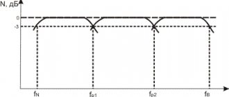
Low-pass filter is a filter that passes without changing frequencies below the cutoff frequency (f0) and suppresses frequencies above f0. At the cutoff frequency it has an amplitude value of -3dB. This is a first order filter and the cutoff slope is 6dB/octave. Most often, such filters are used to cut off high-frequency interference and noise.
An octave is a frequency interval in which the final frequency value is twice as large as the initial frequency.
High Pass Filter (HPF) - also known as a differentiator
A high-pass filter is a filter that attenuates frequencies below the cutoff frequency (f0) and transmits frequencies above f0 without changing. Just like the low-pass filter above, the signal at the cutoff frequency has an amplitude of -3 dB, and a cutoff slope of 6 dB per octave.
Both the low-pass filter and the high-pass filter work as a voltage divider, in which one arm is represented by a constant resistor, and the second by a capacitor, which has a frequency dependence.
Such filters are often used at the outputs of audio amplifiers to cut off infra-low frequencies that can damage speakers.
Radio amateur
Practical calculation of high and low pass filters (RC and LC filters)
Good afternoon, dear radio amateurs! Today, on the “Amateur Radio” website, at the next lesson of the “Beginner Radio Amateur Workshop”, we will look at the procedure for calculating high- and low-pass filters .
From this article you will learn that you can filter not only the “bazaar”, but also much more. And after studying the article, learn how to independently carry out the necessary calculations, which will help you when designing or setting up various equipment (there are a lot of formulas in the article, but it’s not scary, in fact, everything is very simple).
First of all, let’s define that the concepts of
“upper” and “lower” frequencies relate to sound engineering, and the concepts of “high” and “low” frequencies refer to radio engineering.
High-pass filters ( hereinafter referred to as HPF ) and low-pass filters ( hereinafter referred to as LPF ) are used in many electrical circuits and serve different purposes. One of the striking examples of their use is color music devices. For example, if you type “simple color music” in a search engine, you will notice how often the simplest color music on a single transistor is shown in the search results. Naturally, it is very difficult to call such a design color music. Knowing what high- and low-pass filters are and how they are calculated, you yourself can convert such a circuit into a more complete color-music device. The simplest case: you take two identical circuits, but put a filter in front of each. There is a low-pass filter in front of one transistor, and a high-pass filter in front of the second, and you already have two-channel color music. And if you think about it, you can take another transistor and using two filters (low-pass filter and high-pass filter or one medium frequency) to get a third channel - mid-frequency.
Before continuing our conversation about filters, let’s touch on a very important characteristic of them – the amplitude-frequency response ( AFC ). What kind of indicator is this?
The frequency response of a filter shows how the level and amplitude of the signal passing through this filter changes depending on the frequency of the signal. That is, at one frequency of the signal entering the filter, the amplitude level is the same as at the output, and for another frequency, the filter, resisting the signal, weakens the amplitude of the incoming signal.
Another definition immediately appears: cutoff frequency .
The cutoff frequency is the frequency at which the amplitude of the output signal decreases to a value equal to 0.7 from the input. For example, if at an input signal frequency of 1 kHz with an amplitude of 1 volt, the amplitude of the input signal at the filter output is reduced to 0.7 volts, then the frequency of 1 kHz is the cutoff frequency of this filter.
And the last definition is the slope of the filter frequency response .
The slope of the filter's frequency response is an indicator of how sharply the amplitude of the input signal at the output changes when its frequency changes. The faster the frequency response declines, the better.
High- and low-pass filters are ordinary electrical circuits consisting of one or more elements that have a nonlinear frequency response, i.e. having different resistance at different frequencies.
Summarizing the above, we can conclude that in relation to the sound signal, filters are ordinary resistances, with the only difference being that their resistance varies depending on the frequency of the sound signal. This resistance is called reactive and is designated as X.
Frequency filters are made from elements with reactance - capacitors and inductors . The reactance of a capacitor be calculated using the formula below:
Xc=1/2пFC where: Xc is the reactance of the capacitor; p – it is also “pi” in Africa; F – frequency; C is the capacitance of the capacitor. That is, knowing the capacitance of the capacitor and the frequency of the signal, you can always determine what resistance the capacitor has for a specific frequency.
And the reactance of the inductor is given by this formula:
XL=2пFL where: XL is the reactance of the inductor; p – it is also “pi” in Russia; F – signal frequency; L – coil inductance
Frequency filters come in several types: – single-element ; – L-shaped ; – T-shaped ; – U-shaped ; - multi-link .
In this article, we will not delve deeply into theory, but will consider only superficial issues, and only filters consisting of resistances and capacitors (we will not touch filters with inductors).
Single element filter
- a filter consisting of one element : either a capacitor (to highlight high frequencies), or an inductor (to highlight low frequencies).
L-shaped filter
An L-shaped filter is an ordinary voltage divider with a nonlinear frequency response and can be represented as two resistances:
Using a voltage divider, we can reduce the input voltage to the level we need. Formulas for calculating voltage divider parameters:
Uin=Uout*(R1+R2)/R2 Uout=Uin*R2/(R1+R2) Rtot=R1+R2 R1=Uin*R2/Uout – R2 R2=Uout*Rtot/Uin
For example, we are given: Rtot = 10 kOhm , Uin = 10 V , at the output of the divider we need to get Uout = 7 V. Calculation procedure: 1. Determine R2 = 7*10000/10 = 7000 = 7 kOhm 2. Determine R1 = 10* 7000/7-7000= 3000= 3 kOhm, or R1=Rtot-R2=10-7= 3 kOhm 3. Check Uout=10*7000/(3000+7000)= 7 V Which is what we needed. Knowledge of these formulas is necessary not only for constructing a voltage divider with the desired output voltage, but also for calculating low- and high-pass filters, as you will see below.
IMPORTANT! Since the resistance of the load connected to the output of the divider affects the output voltage, the value of R2 should be 100 times less than the input resistance of the load. If high accuracy is not needed, then this value can be reduced up to 10 times. This rule also applies to filter calculations.
To obtain a filter from a voltage divider across two resistors, a capacitor . As you already know, a capacitor has reactance . At the same time, its reactance at high frequencies is minimal, and at low frequencies it is maximum.
When replacing resistance R1 with a capacitor (at high frequencies the current passes through it unhindered, but at low frequencies the current does not pass through it), we get a high-pass filter. And when replacing resistance R2 with a capacitor (at the same time, having a low reactance at high frequencies, the capacitor shunts high-frequency currents to the ground, and at low frequencies its resistance is high and the current does not pass through it) - a low-pass filter.
As I already said, dear radio amateurs, we will not dive deeply into the jungle of electrical engineering, otherwise we will get lost and forget what we were talking about. Therefore, now we will abstract from the complex interrelations of the world of electrical engineering and will consider this topic as a special case, not tied to anything. But let's continue. It's not all bad. Knowledge of at least basic things is a great help in amateur radio practice. Well, we won’t calculate the filter exactly, but we will calculate it with an error. Well, that’s okay, during setup of the device we will select and specify the required ratings of radio components.
Calculation procedure for an L-shaped high-pass filter
In the above examples, the calculation of filter parameters begins with the fact that we know the total resistance of the voltage divider, but it is probably more correct, in the practical calculation of filters, to first determine the resistance of the resistor R2 of the divider, the value of which should be 100 times less than the resistance of the load to which the filter will be connected. And you should also not forget that the voltage divider also consumes current, so in the end, it will be necessary to determine the power dissipation on the resistors for their correct selection.
Example: We need to calculate an L-shaped high pass filter with a cutoff frequency of 2 kHz.
Given : the total resistance of the voltage divider is Rtotal = 5 kOhm , the filter cutoff frequency is 2 kHz . We take the input voltage as 1, and the output voltage as 0.7 (you can take specific voltages, but in our case this does not play any role). We carry out the calculation: 1. Since we connected a capacitor instead of resistor R1 , then the reactance of the capacitor Xc = R1 . R2 using the voltage divider formula : R2=Uout*Rtotal/Uin =0.7*5000/1 = 3500= 3.5 kOhm. 3. Determine the resistance of resistor R1 : R1=Rtotal-R2= 5 – 3.5= 1.5 kOhm. 4. We check the value of the output voltage at the filter output with the calculated resistances: Uout=Uin*R2/(R1+R2) =1*3500/(1500+3500) = 0.7. 5. Determine the capacitance of the capacitor, which is derived from the formula: Xc=1/2пFC=R1 —> C=1/2пFR1: C=1/2пFR1 = 1/2*3.14*2000*1500 =5.3*10- 8 =0.053 µF. The capacitance of the capacitor can also be determined by the formula: C=1.16/R2пF . 6. We check the cutoff frequency Fav using the formula, which we also derive from the above: Fav = 1/2пR1C = 1/2*3.14*1500*0.000000053 = 2003 Hz. Thus, we determined that to build a high-frequency filter with the given parameters (Rtotal = 5 kOhm, Fav = 2000 Hz), it is necessary to use a resistance R2 = 3.5 kOhm and a capacitor with a capacitance C = 0.053 μF. ? For reference: ? 1 µF = 10-6 F = 0.000 001 F? 0.1 µF = 10-7 F = 0.000 000 1 F? 0.01 µF = 10-8 F = 0.000 000 01 F and so on...
Calculation procedure for an L-shaped low-pass filter
Example: We need to calculate an L-shaped low-pass filter with a cutoff frequency of 2 kHz.
Given : the total resistance of the voltage divider is Rtotal = 5 kOhm , the filter cutoff frequency is 2 kHz . We take the input voltage as 1, and the output voltage as 0.7 (as in the previous case). We carry out the calculation: 1. Since we connected a capacitor instead of a resistor R2 , then the reactance of the capacitor Xc = R2 . R2 using the voltage divider formula : R2=Uout*Rtotal/Uin =0.7*5000/1 = 3500= 3.5 kOhm. 3. Determine the resistance of resistor R1 : R1=Rtot-R2= 5 – 3.5= 1.5 kOhm. 4. We check the value of the output voltage at the filter output with the calculated resistances: Uout=Uin*R2/(R1+R2) =1*3500/(1500+3500) = 0.7. 5. Determine the capacitance of the capacitor, which is derived from the formula: Xc=1/2пFC=R2 —> C=1/2пFR2: C=1/2пFR2 = 1/2*3.14*2000*3500 =2.3*10- 8 =0.023 µF. The capacitance of the capacitor can also be determined by the formula: C=1/4.66*R2pF . 6. We check the cutoff frequency Fav using the formula, which we also derive from the above: Fav = 1/2пR2C = 1/2*3.14*3500*0.000000023 = 1978 Hz. Thus, we determined that to build a low-pass filter with the given parameters (Rtotal = 5 kOhm, Fav = 2000 Hz), it is necessary to use a resistance R1 = 1.5 kOhm and a capacitor with a capacitance C = 0.023 μF.
T-shaped filter
T-shaped high-pass and low-pass filters are the same L-shaped filters, to which one more element is added. Thus, they are calculated in the same way as a voltage divider consisting of two elements with a nonlinear frequency response. And then, the reactance value of the third element is added to the calculated value. Another, less accurate way of calculating a T-shaped filter begins with calculating the L-shaped filter, after which the value of the “first” calculated element of the L-shaped filter is increased or decreased by half - “distributed” between two elements of the T-shaped filter. If it is a capacitor, then the value of the capacitance of the capacitors in the T-filter is doubled, and if it is a resistor or inductor, then the value of the resistance or inductance of the coils is halved:
U-shaped filter
U-shaped filters are the same L-shaped filters, to which another element is added in front of the filter. Everything that was written for T-shaped filters is true for U-shaped ones. As in the case of T-shaped filters, to calculate U-shaped filters, voltage divider formulas are used, with the addition of an additional shunt resistance of the first filter element. Another, less accurate method of calculating a U-shaped filter begins with calculating the L-shaped filter, after which the value of the “last” calculated element of the L-shaped filter is increased or decreased by half - “distributed” between two elements of the U-shaped filter. In contrast to the T-shaped filter, if it is a capacitor, then the value of the capacitance of the capacitors in the P-filter is halved, and if it is a resistor or inductor, then the value of the resistance or inductance of the coils is doubled.
As a rule, single-element filters are used in acoustic systems. High-pass filters are usually made T-shaped, and low-pass filters are U-shaped. Mid-pass filters, as a rule, are made L-shaped, consisting of two capacitors.
To write the article, among other things, we used materials from the website www.meanders.ru, the author and owner of which is Alexander Melnik, for which we thank him very much and endlessly (Meanders).