What is a low pass filter? Passive rc filter basics guide

INTRODUCTION

In our time of high technology, nonlinear loads (frequency converters, inverters, uninterruptible power supply systems, switching power supplies, fluorescent and LED lamps, etc.) are becoming more and more common. Because of these changes in load patterns, power quality and harmonic mitigation have become major topics this decade. Problems caused by harmonics, such as overheating of transformers and rotating machines, overloading of neutral conductors, failure of capacitor banks, etc., lead to increased operating costs and can also lead to a decrease in product quality and labor productivity. In addition, changes in the electricity generation mix towards wind and solar power, which also generate harmonics, also mean that the use of harmonic filters is becoming increasingly important to ensure a stable power supply with acceptable power quality.

The level of harmonics can be reduced using passive filters (composed of capacitors, reactors and resistors) or active filters (generating harmonics in antiphase to distortion harmonics and thereby destroying them)

Although the basic principles of active filters were developed back in the 1970s, they have received increased attention in the last few years because of the availability of insulated gate bipolar transistors (IGBTs) and digital signal processors (DSPs). At the same time, the cost difference between active and passive filters is not as large as in the past

This article compares the advantages and disadvantages of active and passive filtration technologies. Passive and active solutions for harmonic mitigation and network stabilization are discussed to address problems that arise in current applications and are likely to arise in the future.

Influence of the filter on the phase response

The influence of the filter on the phase response of the signal is no less significant than its influence on the frequency response. For audio signals, the effect of the filter's phase response on the signal can be decisive when choosing the filter type.

Apart from the active element (transistor or microcircuit), active filters are usually built on RC circuits. Each RC circuit is a filter pole that bends the frequency response in the direction we need. But at the same time, each RC circuit introduces a finite time delay into the signal.

This delay causes the signal after the filter to be phase shifted relative to the original signal. The whole problem is that this delay can be different for different frequencies.

This applies to any filter . But the difference between the types of filters is that they have different phase-frequency characteristics and different cutoff slopes.

Electromagnetic compatibility of frequency converters

Electromagnetic compatibility of technical equipment is the normal (with the required quality) performance of technical equipment in a real environment despite unintentional exposure to electromagnetic interference and the ability not to create unacceptable interference with other equipment.

All models of vector frequency converters are equipped with line filters, which ensures the required level of EMC. Filters may not be used in the range up to 30 kW. All higher power frequency converters are equipped with built-in filters by default. The built-in filter makes it possible to minimize interference and interference in electronic equipment.

Crossover Frequency

Now is the time to think about the frequency of the section. Typically, the crossover frequency is selected in flat horizontal areas, away from resonances and blockages, trying to avoid sudden irregularities as potential sources of distortion... And if you remember that there is a phase about which little is known, and if it is known, then you can’t add up the vector frequency response on a piece of paper, but from - due to the curvature of the phases, even on a perfectly flat frequency response, something will come out, something will fail to a greater or lesser extent. You also need to remember what the speaker itself, especially the high frequency, can provide; for example, you shouldn’t force an inch dome to play from two, much less one, kilohertz, even if it is capable of playing them back according to the frequency response.

So, let's look at what unique speakers we got. The high-frequency driver begins to fall at 1.3 kHz, which means it cannot be allowed lower. On the other hand, the subwoofer tries to play at as low as 10 kHz, with varying degrees of success. However, common sense dictates that launching it above kilohertz is a bad idea. And what should you do if the operating ranges of the speakers do not intersect?

There are two options: if the declines have an adequate steepness, then it is best to drive into a hole, especially if the hole turns out to be wide. In our case, when the declines are as steep as cliffs, we must stay away from the steepest of them. Most often, this can happen with a high-frequency driver; it is always difficult for them to work at the lower limit of the range, so it is more expedient for them to make their life easier by entrusting the reproduction of the lower part of the range to a low-frequency speaker, which will play at least poorly, but will not spoil. Therefore, we limit the range to the area from 1.5 kHz to 2.2 kHz.

Speaker phasing

This brings the mixing to an end. All that remains is to decide on the phasing of the speakers. There are at least three ways: by ear, by the shape of the frequency response and by the phase shift at the crossover frequency. If the speakers have a moderately linear frequency response and phase response, and the filter does not greatly increase the phase at the crossover, then when the correct phase changes to an incorrect one, a deep dip will appear at the crossover frequency, it is difficult to miss it. In this case, it is worth adjusting the phase according to its shift. This can be done with an oscilloscope by feeding the horizontal deflection signal from the amplifier, and the vertical deflection signal from the microphone.

A sine wave with the crossover frequency is supplied to the amplifier input and, without changing the relative position of the microphone and speakers, the high-frequency and low-frequency speakers are switched. Based on the similarity of the Lissajous figures, a conclusion is drawn about the equality of the phases of the emitters. This method works well for first order filters. With the curvature of our speakers, this method does not justify itself, so we compare the frequency response at different phasing.

The second option is noticeably worse. However, the first one is not the ultimate dream, but since moving the inductance of the coils is not easy, and it’s too lazy to tinker further, everything was left as is.

Filter order

Usually, when the question arises about creating a filter, the first step is to decide what slope slope is needed. It directly determines the filter order. The higher the order of the low-pass filter, the steeper the frequency response will roll off above the cutoff frequency.

For convenience, this and subsequent graphs show the normalized frequency. Those. as if all frequencies were divided by the filter cutoff frequency.

But the higher the order of the filter, the more difficult it will be to implement and the more capricious to configure. Moreover, the higher the order, the worse the effect it will have on the frequency and/or phase characteristics of the signal.

Usually, when a high-order filter is needed, to simplify circuit design and calculations, they resort to sequential connection of two, three or more second-order filters. This, of course, makes the task easier, but with this connection, either different gains of each filter or different cutoff frequencies are required. But this is beyond the scope of this article.

Calculation of the amplitude-frequency response of the filter

We can calculate the theoretical behavior of a low-pass filter using a frequency-dependent version of a typical voltage divider calculation. The output voltage of a resistive voltage divider is expressed as follows:

Figure 9 – Resistive voltage divider

An RC filter uses an equivalent structure, but instead of R2 we have a capacitor. First we replace R2 (in the numerator) with the reactance of the capacitor (XC). Next we need to calculate the value of the impedance and place it in the denominator. Thus we have

The reactance of a capacitor indicates the amount of resistance to the flow of current, but, unlike active resistance, the amount of resistance depends on the frequency of the signal passing through the capacitor. So we have to calculate the reactance at a certain frequency and the formula we use for this is the following:

In the example circuit above, R ≈ 160 ohms, and C = 10 nF. Let's assume that the amplitude of Vin is 1 V, so we can simply remove Vin from the calculations. First, let's calculate the amplitude of Vout at the frequency of the sinusoid we need:

The amplitude of the sinusoidal signal we need practically does not change. This is good since we intended to preserve the sine wave while suppressing noise. This result is not surprising since we chose a cutoff frequency (100 kHz) that is much higher than the frequency of the sine wave (5 kHz).

Now let's see how successfully the filter will attenuate the noise component.

The noise amplitude is only about 20% of the original value.

Classification of filters according to the type of their amplitude-frequency characteristics

Low pass filters. Low-pass filters (LPFs) are characterized by the fact that low-pass input signals, starting with constant signals, are transmitted to the output, and high-frequency signals are delayed. In Fig. 12.1, a

the characteristic of an ideal (not implemented in practice) filter is shown (it is sometimes called the “brick wall” type characteristic). Other figures show the characteristics of real filters.

Rice. 12.1. Amplitude-frequency characteristics

low pass filters

The passband ranges from zero frequency to cutoff frequency ωс

.
Typically, the cutoff frequency is defined as the frequency at which the value of A( ω
) is equal to 0.707 of the maximum value (i.e., 3
dB
).

The stop band (suppression) starts from the stop frequency ωз

and continues ad infinitum.
In some cases, the delay frequency is defined as the frequency at which the value of A( ω
) is 40
dB
(i.e., 100 times less).

Between the passband and stopband of real filters there is a transition band. An ideal filter has no transition frequency.

High pass filters. A high-pass filter is characterized by the fact that it passes high-pass signals and delays low-pass signals.

In Fig. 12.2, a

the ideal (unrealizable) amplitude-frequency response of a low-pass filter is shown, and in Fig.
12.2, b
- one of the typical real ones.
by ωс
and
ωз
.

Rice. 12.2. Amplitude-frequency characteristics

high pass filters

Bandpass filters (bandpass). A bandpass filter passes signals from one frequency band located in some inner part of the frequency axis. Signals with frequencies outside this band are blocked by the filter.

In Fig. 12.3, a

The amplitude-frequency characteristic of an ideal (impracticable) filter and one of the typical real characteristics are shown (Fig. 12.3,
b
).

Two cutoff frequencies are designated
by ωс1
and
ωс2 ω0
is the average frequency. It is defined by the expression

Rice. 12.3. Amplitude-frequency characteristics of a bandpass filter

A-

ideal characteristic;
b-
real characteristic

Notch filters (band-stop). Notch filters do not transmit (delay) signals lying in a certain frequency band, and transmit signals with other frequencies.

The amplitude-frequency response of an ideal (unrealizable) filter is shown in Fig. 12.4, a

.
In Fig. Figure 12.4, b
shows one of the typical real characteristics.

Rice. 12.4. Amplitude-frequency characteristics

notch filter

All-pass filters (phase correctors). These filters pass signals of any frequency. Such filters are used in some electronic systems in order to change the phase-frequency characteristic of the entire system for one purpose or another (Fig. 12.5).

Rice. 12.5. Amplitude-frequency response

all-pass filter

Classification of filters by transfer functions using the example of low-pass filters. In practice, filters that differ in their characteristic amplitude-frequency characteristics are widely used. These are Butterworth, Chebyshev, Bessel (Thomson) filters (Fig. 12.6).

Rice. 12.6. Amplitude-frequency characteristics of filters

Butterworth filters are characterized by the flattest amplitude-frequency response in the passband. This is their dignity. But in the transition zone, these characteristics decrease smoothly, not sharply enough.

Chebyshev filters are characterized by a sharp decrease in amplitude-frequency characteristics in the transition band, but in the passband these characteristics are not flat.

Bessel filters are characterized by very flat sections of the amplitude-frequency characteristics in the transition band, even flatter than those of Butterworth filters. Their phase-frequency characteristics are quite close to ideal, corresponding to a constant deceleration time, so such filters little distort the shape of the input signal containing several harmonics.

the characteristic of an ideal (not implemented in practice) filter is shown (it is sometimes called the “brick wall” type characteristic). Other figures show the characteristics of real filters.

Rice. 12.1. Amplitude-frequency characteristics

low pass filters

The passband ranges from zero frequency to cutoff frequency ωс

.
Typically, the cutoff frequency is defined as the frequency at which the value of A( ω
) is equal to 0.707 of the maximum value (i.e., 3
dB
).

The stop band (suppression) starts from the stop frequency ωз

and continues ad infinitum.
In some cases, the delay frequency is defined as the frequency at which the value of A( ω
) is 40
dB
(i.e., 100 times less).

Between the passband and stopband of real filters there is a transition band. An ideal filter has no transition frequency.

High pass filters. A high-pass filter is characterized by the fact that it passes high-pass signals and delays low-pass signals.

In Fig. 12.2, a

the ideal (unrealizable) amplitude-frequency response of a low-pass filter is shown, and in Fig.
12.2, b
- one of the typical real ones.
by ωс
and
ωз
.

Rice. 12.2. Amplitude-frequency characteristics

high pass filters

In Fig. 12.3, a

Rice. 12.3. Amplitude-frequency characteristics of a bandpass filter

A-

ideal characteristic;
b-
real characteristic

Notch filters (band-stop). Notch filters do not transmit (delay) signals lying in a certain frequency band, and transmit signals with other frequencies.

The amplitude-frequency response of an ideal (unrealizable) filter is shown in Fig. 12.4, a

.
In Fig. Figure 12.4, b
shows one of the typical real characteristics.

Rice. 12.4. Amplitude-frequency characteristics

notch filter

Rice. 12.5. Amplitude-frequency response

all-pass filter

Rice. 12.6. Amplitude-frequency characteristics of filters

Chebyshev filters are characterized by a sharp decrease in amplitude-frequency characteristics in the transition band, but in the passband these characteristics are not flat.

Bandpass Resonant Filters

Band-pass resonant frequency filters are designed to isolate or reject (cut out) a certain frequency band. Resonant frequency filters can consist of one, two, or three oscillatory circuits tuned to a specific frequency. Resonant filters have the steepest rise (or fall) in the frequency response compared to other (non-resonant) filters. Band-pass resonant frequency filters can be single-element - with one circuit, L-shaped - with two circuits, T and U-shaped - with three circuits, multi-element - with four or more circuits.

The figure shows a diagram of a T-shaped bandpass resonant filter designed to isolate a certain frequency. It consists of three oscillatory circuits. C.L.

and
CL
- series oscillatory circuits, at the resonant frequency they have low resistance to the flowing current, and at other frequencies, on the contrary, they have high resistance.
The CL
parallel circuit , on the contrary, has a high resistance at the resonant frequency, but has low resistance at other frequencies.
To expand the bandwidth of such a filter, the quality factor of the circuits is reduced by changing the design of the inductors, detuning the circuits “right, left” to a frequency slightly different from the central resonant one, and a resistor is connected in parallel with the CL
.

The following figure shows a diagram of a T-shaped notch resonant filter designed to suppress a specific frequency. It, like the previous filter, consists of three oscillatory circuits, but the principle of frequency selection for such a filter is different. C.L.

and
CL
- parallel oscillatory circuits, at the resonant frequency they have a large resistance to the flowing current, and at other frequencies - small.
The CL
parallel circuit , on the contrary, has low resistance at the resonant frequency, but has high resistance at other frequencies. Thus, if the previous filter selects the resonant frequency and suppresses the remaining frequencies, then this filter freely passes all frequencies except the resonant frequency.

The procedure for calculating bandpass resonant filters is based on the same voltage divider, where the LC circuit with its characteristic resistance acts as a single element. How an oscillatory circuit is calculated, its resonant frequency, quality factor and characteristic (wave) impedance are determined, you can find in the article Oscillating circuit.

Chebyshev filter and sound?

Let's start with the Chebyshev filter. It has the sharpest frequency response rolloff. But the phase shift it introduces varies greatly throughout the entire passband. For this reason, the Chebyshev filter is not used in high-quality audio circuits.

But this is not the only disadvantage. The Chebyshev filter also has a large frequency response unevenness in the passband. In this case, the sum of the maxima and minima is equal to the order of the filter

The following graph shows the amplitude-frequency (left scale) and phase-frequency (right scale) characteristics for an 8th order Chebyshev filter. The same is true for Chebyshev filters of lower orders.

System sound

And of course we must say about the sound. It got better, the scene turned out very good. The curvature of the frequency response is not particularly audible; on the contrary, the rise in the middle lends itself to detail; oddly enough, there is enough highs. An interesting effect was noticed on the bass. As you can see from the frequency response at a hundred hertz there is a big rise, followed by a drop, of course there is no pumping bass, but there is mid bass. For example, the guitar part seems a little lost, but the lower bass, the bass guitar part, seems to move into the audible area and is read very clearly, giving the impression of having that same low bass.

Of course, the boxes are too small, and sometimes you can hear the muttering, to eliminate this effect, 30 grams of natural wool were added to each column. In general, this acoustics plays warmly and softly even without a tube amplifier, maintaining the rigor and precision of stone in the sound, but with a warm tube it turns out to be too soft. Still, they need a stricter amplifier - a triode or push-pull, but this is a topic for the next experiments. Especially for the Radio Circuits website - SecretTUseR.

Discuss the article FILTER FOR ACOUSTICS

Practical work

We smoothly move from theory to practice. I got vintage speakers called Kompaktbox B 9251. And the first thing that was done was listening.

With a cold stone, the sound was on average not bad, and if we speak specifically, in some places it was good, but in others it was haphazard. They refused to play with a warm lamp at all. Based on these observations, it was concluded that there was deep buried potential. An autopsy showed that German engineers decided to make do with one single capacitor in series with the RF head. The frequency response measurement gave a terrible picture

In the figure, the frequency response of one speaker, a curve with a deep hole at 6 kHz due to poor connector contact, do not pay attention to it. The frequency response separately for HF and LF is given below

T-shaped high and low pass filters

T-shaped high- and low-pass filters are the same L-shaped filters, to which one more element is added. Thus, they are calculated in the same way as a voltage divider consisting of two elements with a nonlinear frequency response. And then, the reactance value of the third element is added to the calculated value. Another, less accurate way of calculating a T-shaped filter begins with calculating the L-shaped filter, after which the value of the “first” calculated element of the L-shaped filter is increased or decreased by half - “distributed” between two elements of the T-shaped filter. If it is a capacitor, then the value of the capacitance of the capacitors in the T-filter is doubled, and if it is a resistor or inductor, then the value of the resistance or inductance of the coils is halved. The transformation of filters is shown in the figures. The peculiarity of T-shaped filters is that, compared to L-shaped ones, their output resistance has a lower shunting effect on the radio circuits behind the filter.

Converting an L-shaped RC high-pass filter into a T-shaped RC high-pass filter Converting an L-shaped RC low-pass filter into a T-shaped RC low-pass filter Converting an L-shaped RL high-pass filter into a T-shaped RL high-pass filter frequencies Conversion of an L-shaped RL low-pass filter into a T-shaped RL low-pass filter Conversion of an L-shaped LC high-pass filter into a T-shaped LC high-pass filter Conversion of an L-shaped LC low-pass filter into a T-shaped LC filter low frequencies

U-shaped filter

U-shaped filters are the same L-shaped filters, to which another element is added in front of the filter. Everything that was written for T-shaped filters is true for U-shaped ones. As in the case of T-shaped filters, to calculate U-shaped filters, voltage divider formulas are used, with the addition of an additional shunt resistance of the first filter element. Another, less accurate method of calculating a U-shaped filter begins with calculating the L-shaped filter, after which the value of the “last” calculated element of the L-shaped filter is increased or decreased by half - “distributed” between two elements of the U-shaped filter. In contrast to the T-shaped filter, if it is a capacitor, then the value of the capacitance of the capacitors in the P-filter is halved, and if it is a resistor or inductor, then the value of the resistance or inductance of the coils is doubled.

As a rule, single-element filters are used in acoustic systems. High-pass filters are usually made T-shaped, and low-pass filters are U-shaped. Mid-pass filters, as a rule, are made L-shaped, consisting of two capacitors.

SAY A WORD ABOUT THE POOR SQUEEER

A.I. Shikhatov 2003

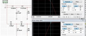
Traditionally, the separation of the midrange and high-frequency bands (or midbass-HF) is carried out by passive crossovers (separation filters). This is especially convenient when using ready-made component kits. However, although the characteristics of crossovers are optimized for a given set, they do not always satisfy the task. An increase in voice coil inductance with frequency leads to an increase in head impedance. Moreover, this inductance for the “average” midbass is 0.3-0.5 mH, and already at frequencies of 2-3 kHz the impedance almost doubles. Therefore, when calculating passive crossovers, two approaches are used: they use the real impedance value at the crossover frequency in the calculations or introduce impedance stabilization circuits (Zobel compensators). A lot has already been written about this, so we won’t repeat it. Squeakers usually do not have stabilizing chains. In this case, it is assumed that the operating frequency band is small (two to three octaves), and the inductance is insignificant (usually less than 0.1 mH). As a result, the increase in impedance is small. In extreme cases, the increase in impedance is compensated by a 5-10 Ohm resistor connected in parallel to the tweeter. However, everything is not as simple as it seems at first glance, and even such a modest inductance leads to interesting consequences. The problem is that the tweeters work in conjunction with the high-pass filter. Regardless of the order, it contains a capacitance connected in series with the tweeter, and it forms an oscillatory circuit with the inductance of the voice coil. The resonance frequency of the circuit turns out to be in the operating frequency band of the tweeter, and a “hump” appears on the frequency response, the magnitude of which depends on the quality factor of this circuit. As a result, sound coloration is inevitable. Recently, many models of high-sensitivity tweeters (92 dB and higher) have appeared, the inductance of which reaches 0.25 mH. Therefore, the issue of matching a tweeter with a passive crossover becomes especially acute. The Micro-Cap 6.0 simulation environment was used for the analysis, but the same results can be obtained using other programs (Electronic WorkBench, for example). Only the most typical cases are given as illustrations; the remaining recommendations are given at the end of the article in the form of conclusions. The calculations used a simplified model of the tweeter, taking into account only its inductance and active resistance. This simplification is quite acceptable, since the resonant impedance peak of most modern tweeters is small, and the mechanical resonance frequency of the moving system is outside the operating frequency band. Let us also take into account that the frequency response for sound pressure and the frequency response for electrical voltage are two big differences, as they say in Odessa. The interaction of the tweeter with the crossover is especially noticeable in first-order filters, typical of inexpensive models (Figure 1):

Picture 1

It can be seen that even with an inductance of 0.1 mH there is a pronounced peak in the frequency range of 7-10 kHz, giving the sound a characteristic “crystal” coloring.” Increasing the inductance shifts the resonant peak to lower frequencies and increases its quality factor, which leads to a noticeable “clunking”. A side effect of an increase in quality factor, which can be turned to benefit, is an increase in the slope of the frequency response. In the region of the crossover frequency, it is close to 2nd order filters, although at a large distance it returns to the original 1st order value (6 dB/octave). The introduction of a shunt resistor allows you to “tame” the hump on the frequency response, so that some equalizer functions can be assigned to the crossover. If the shunt is made on the basis of a variable resistor (or a set of resistors with a switch), then you can even quickly adjust the frequency response within 6-10 dB. (Figure 2):

Figure 2

However, first-order filters provide too little attenuation outside the operating band, so they are only suitable for low input power or a sufficiently high crossover frequency (7-10 kHz). Therefore, in most serious designs, filters of higher orders are used, from the second to the fourth. Let's consider the possibilities of influencing the frequency response for second-order filters, as the most common. For clarity, a model with high inductance is used. The same results are obtained with traditional tweeters, only the filter parameters and the degree of influence on the frequency response will be different. For tweeters with low inductance, a shunt is not necessary. The first method is to change the quality factor of the filter at a constant crossover frequency due to the ratio of the capacitance and inductance of the filter (Figure 3):

Figure 3

Simultaneously changing capacitance and inductance in a crossover is difficult, so this method is inconvenient for operational adjustment. However, it is indispensable in cases where the required degree of correction is known in advance, at the design stage.

The second method is to adjust the quality factor using a shunt (similar to the previously discussed method for a first-order filter). The initial quality factor of the separating filter is selected high (Figure 4):

Figure 4

The third method is to introduce a resistor in series with the tweeter. This method is especially convenient for tweeters with inductance over 100 mH. In this case, the total impedance of the “resistor-tweeter” circuit changes slightly during the regulation process, so the signal level practically does not change (Figure 5):

Figure 5

Conclusions Stabilizing circuits are not necessary only for tweeters with low inductance (less than 0.05 mH). For tweeters with a voice coil inductance of 0.05-0.1 mH, parallel stabilizing circuits (shunts) are most advantageous. For tweeters with a voice coil inductance greater than 0.1 mH, both parallel and series stabilizing circuits can be used. Changing the resistance of the stabilizing circuit allows you to influence the frequency response. For 1st order filters, changing the parameters of the stabilizing circuit has a noticeable effect on the cutoff frequency and hump parameters. For 2nd order filters, the cutoff frequency is determined by the parameters of its elements and depends to a lesser extent on the inductance of the head and the parameters of the stabilizing circuit. The magnitude of the resonant “hump” caused by the inductance of the tweeter is directly dependent on the resistance of the shunt and inversely related to the resistance of the series resistor. The magnitude of the resonant “hump” in the region of the cutoff frequency is directly dependent on the quality factor of the filter. The quality factor of the filter is proportional to the resulting load resistance (RF head taking into account the resistance of the stabilizing circuit). A high-quality filter can be calculated using the standard method, but for a load resistance reduced by 2-3 times relative to the nominal load resistance.

The proposed methods for regulating the frequency response are also applicable to filters of higher orders, but since the number of “degrees of freedom” there increases, it is difficult to give specific recommendations in this case. An example of changing the frequency response of a third-order filter due to a shunt resistor is shown in Figure 6:

Figure 6

It can be seen that the frequency response takes on a different appearance, which significantly affects the sound timbre. By the way, about 20 years ago, many “home” three or four-way speakers had switchable frequency response “normal/crystal/chirp” (“smooth-crystal-chirp”). This was achieved by changing the level of the mid and high frequency bands. Switchable attenuators are used in many crossovers, and in relation to the tweeter they can be considered a combination of series and parallel stabilizing circuits. Their impact on the resulting frequency response is quite difficult to predict; in this case, it is more convenient to resort to modeling.

Figure 7

Figure 7 shows the diagram and frequency response of a third-order filter developed by the author for the Prology RX-20s and EX-20s tweeters. The design uses K73-17 capacitors (2.2 µF, 63 V) and homemade inductors. To reduce active resistance, they are wound on ferrite rings. The type of core is unknown: outer diameter 15 mm, magnetic permeability of the order of 1000-2000. Therefore, the inductance adjustment was carried out using the F-4320 device. Each coil contains 13 turns of insulated wire with a diameter of 1 mm. The sound quality turned out to be much higher than the original one, and the frequency response regulation was fully consistent with the task. However, it should be noted that the filter turned out to be problematic: the input impedance has a pronounced minimum, and the amplifier’s protection may be triggered.

Site administration address

DON'T FIND WHAT YOU WERE LOOKING FOR? GOOGLE:

CUSTOM SEARCH STRING

WAYS TO REDUCE HARMONICS LEVEL

Possible ways to mitigate harmonics are, for example, increasing the short-circuit current of the network (reducing the network impedance), limiting the capacity / number of simultaneously operating harmonic sources, balancing single-phase loads on three phases and using equipment with a higher pulsation (for example, using 12- or 18-pulse frequency converter instead of 6-pulse). However, the most common solutions are the use of a passive filter consisting of a combination of capacitors, inductances and resistances (RC, RL, LC, LCQ and others), as well as active filters that are becoming increasingly widespread. Hybrid solutions (combinations of active and passive filters) are also used.

When using a passive resonant filter, its circuit is tuned to a specific frequency, that is, the resonant frequencies of the series filter are very close to the frequencies of the existing harmonics. When designing a resonant filter, a careful analysis of the load and power quality is of great importance, and the value of the network impedance is also very important (Figure 2).

Rice. 2. Dependence of system busbar impedance on frequency

As shown in Figure 3, the switching sequence is important for resonant filtering, it must follow the LIFO (last in first out) rule, the opposite can lead to problems.

Rice. 3. Sequence of switching resonant filters in accordance with the LIFO rule

A) Example: using a resonant filter

The real example below (Figures 4, 5) shows a resonant filter for the 5th and 7th harmonics. It is installed in a shopping mall in China.

Rice. 4. Electrical diagram for connecting a resonant filter in a shopping center in China

The filter analysis results are shown in Figure 5. It can be seen that not only the 5th and 7th harmonic currents are reduced, but also the voltage harmonic distortion is reduced from 4.8% to 1.8%. The power factor also increased from 0.92 to 0.99.

RESONANCE FILTERS	Result/reduction
Without a filter	1 5th harmonic filter (1) incl.	2nd 5th harmonic filter (2) on.	7th harmonic filter (3) on.
11:09:30	11:10:00	11:11:00	11:11:30
Active power, kW	P	1489	1494	1497	1506
Reactive power, kvar	Q	641	364	188	190	70,36%
Apparent power, kVA	S	1621	1538	1509	1518	6,35%
Voltage, V	U	234	235,567	237,075	238,867	2,08%
Valid current value, A	Irms	2266	2109	2050	2078	8,30%
Harmonic distortion factor	THD-V	4,78%	3,04%	2,79%	1,78%	62,82%
5th harmonic voltage	HRU5	3,83%	0,89%	0,81%	0,94%	75,38%
7th harmonic voltage	HRU7	1,77%	2,32%	2,15%	0,89%	49,49%
11th harmonic voltage	HRU11	1,40%	0,89%	0,86%	0,62%	56,00%
Current harmonic distortion factor	THD-I	17,68%	394.51 A	9,92%	208.25 A	9,93%	202.51 A	6,56%	135.94 A	65,54%
5th harmonic current	HRI5	16,21%	361.71 A	3,85%	80.82 A	4,31%	87.90 A	5,12%	106.17 A	70,65%
7th harmonic current	HRI7	4,68%	104.43 A	8,16%	171.19 A	7,99%	163.03 A	2,75%	56.98 A	45,44%
11th harmonic current	HRI11	3,38%	75.47 A	2,30%	48.31 A	1,87%	38.23 A	1,13%	23.33 A	69,09%
Fundamental current	I1	2231	2099	2040	2074	7,07%
Power factor	PF	0,92	0,97	0,99	0,99

Rice. 5. Results of applying a resonant filter in a shopping center in China

B) Advantages and disadvantages of passive filters

How to assemble a low pass filter

Instructions on how to properly make a low-pass filter are useful for many. In radio engineering it is always necessary to produce filters of different heights. And making your own low-pass filter is not that difficult.

Here's what you need to make a low-pass filter:

Various parts for soldering to a printed circuit board.
Fiberglass for printed circuit boards.
Current source.
The soldering iron is simple.

Next, we print out the drawing of the tracks for the board and transfer it to our workpiece.

If the paths are not clear, they should be completed using varnish. After everything has been transferred, you need to clean the board using a special solution.

You can create a solution from citric acid and hydrogen peroxide. They are mixed in a ratio of 1:3, respectively. To make the solution act faster, a catalyst is added - salt on the tip of a knife.

As soon as the solution is ready, the board is placed in it and the time is waited until it is completely cleaned. The copper that remains on the surface of the tracks should completely dissolve. After cleaning the board, rinse it under running water.

Once the process is complete, you can begin soldering the parts. In order to do everything accurately, refer to the video master class on soldering parts.

So you've noticed how easy it is to create your own low-pass filter. Using the same principle, you can independently come up with a circuit for manufacturing a high-frequency filter.

Active crossovers for speakers based on a 3rd order Butterworth filter

Hello everyone, In order not to have difficulties with calculating the MF-HF filter, it may seem correct to use the so-called additional function filter (AFF) - a differential amplifier that subtracts from the broadband (musical) signal that which was isolated by the low-pass filter (in in our case), and the remainder is the midrange and high-frequency components, which are transmitted to its output.

Practical schemes of crossovers with FDF are described in detail in the articles of Radio magazine: 1981 No. 5-6 page 39 “Three-band amplifier” 1987 No. 3 page 35 “Filter block of three-band AF amplifier”

Please note that in the '87/3 circuit, in front of the active filter there is a voltage follower on the op-amp, which follower has a low output impedance, and the filter on the op-amp (FDF) with a high input impedance is loaded, which is useful for matching the filter with the circuit forming the crossover, generally.

It is better to choose a crossover frequency for a two-way crossover that is three times greater than the resonant frequency of the woofer. If a full-range speaker is used as a low-frequency loudspeaker, then it is better to conduct the section above 3.5 KHz (above the resonant frequency of the selected high-frequency loudspeaker). A table linking the crossover frequency during bi-ampling with the power that needs to be supplied to the mid-frequency - high-frequency link is given in Radio 2001 No. 9, page 10

Before this crossover, it would be good to put a high-pass filter with a cutoff frequency of 40 Hz or less - cut off what your woofer cannot physically reproduce. This is described in detail at Audiokiller electroclub.info/samodel/sub_pred.htm

An article on measuring the resonant frequency of loudspeakers and their “T-C parameters” using a computer sound card is available here on the website. datagor.ru/practice/loudspeakers/1366-izmerenie-parametrov-tilya-smolla-dlya-nachinayushhix.html

On the topic of two-way sound reproduction (biampling), it is interesting to read the article by V. Shorov from Radio 1994 No. 2 “Two-way sound reproduction” and, if you want to understand better, the series of articles by A. Frunze “On improving the sound quality of speakers” Radio 1992 9 - 12.

I would like to thank AudioKiller for the program for calculating third-order filters. electroclub.info/mysoft.htm Based on the calculations performed, I assembled a combined (on one op-amp) bandpass filter 40 - 18000 Hz for a VHF receiver. With precise selection of capacitors and resistors, the frequency response of the filter coincided with the desired one without additional adjustment.

Beginners who have successfully assembled a circuit layout can save themselves the hassle of etching printed circuit boards by using non-foil fiberglass (getinax or thick cardboard) and thin tinned wire that replaces the traces that were supposed to be etched. In the LayOut program, a printed circuit board is drawn with a track width of 0.3 - 05 mm. - to be visible. Based on the printout of the board design, protected with transparent tape, the PCB is cored and drilled. Then parts are inserted into the holes, according to the assembly order, from the entrance to the exit, their tinned leads are bent in the direction of the drawn tracks and soldered. If the leads are not long enough, use tinned wire. If the conductors - “paths” - lie close to each other and there is a risk of short circuiting, you can put on a cambric. It is important that if rework is required, for example, 20% of the assembled circuit, you do not need to cut off the printed tracks - just unsolder the section, make a new drill and reassemble - clean, simple and technologically, like paving slabs. When assembling HF structures, the foil layer facing the parts can be used as a general shield. The foil around the holes must be countersunk, except for the “ground” contacts. If you're interested, I'll send you photos of boards made this way.

Effect of interference on drive equipment

In industry, the majority of power consumption is accounted for by fans, pumps, compressors, conveyors and winches, and drives of process units. The mechanical part of this entire facility is driven by AC asynchronous motors. Mode control of the operation of asynchronous motors, including reduction of their electricity consumption, is carried out using specialized devices - frequency converters. Their benefit lies in significantly facilitating the starting modes and operation of directly asynchronous motors. However, sometimes frequency converters have an undesirable effect on the engine.

Due to the special design of the frequency converter, its output voltage and current have the form of a burst with a huge amount of noise. The rectifier of the converting device, consuming nonlinear current, creates higher harmonics, thereby polluting the electrical network. Frequency converter inverter (PWM) – generates a wide range of high-frequency harmonics.

Power supply to the motor windings with such non-standard current sometimes leads to thermal and electrical breakdown of the insulation of the motor windings, wear of the insulation, an increase in the degree of acoustic noise of the operating motor, and erosion of bearings. In addition, frequency converters generate noise in the electrical network, which has a negative impact on other electrical equipment powered from the same electrical network. To reduce the adverse effect of harmonic distortion generated by the frequency converter during operation on the electrical network, filtering is used for the motor and the frequency converter itself.

Single element high and low pass filters

As a rule, single-element high- and low-pass filters are used directly in the acoustic systems of powerful audio amplifiers to improve the sound of the audio speakers themselves.

They are connected in series with the dynamic heads. Firstly, they protect both the dynamic heads from a powerful electrical signal and the amplifier from low load resistance without loading it with extra speakers at a frequency that these speakers do not reproduce. Secondly, they make playback more pleasant to the ear.

To calculate a single-element filter, you need to know the reactance of the dynamic head coil. The calculation is made using the voltage divider formulas, which is also true for an L-shaped filter. Most often, single-element filters are selected “by ear”. To highlight high frequencies on the tweeter, a capacitor is installed in series with it, and to highlight low frequencies on a low-frequency speaker (or subwoofer), a choke (inductor) is connected in series with it. For example, with powers of the order of 20...50 Watts, it is optimal to use a 5...20 µF capacitor for tweeters, and as a choke for a low-frequency speaker, use a coil wound with enameled copper wire, 0.3...1.0 mm in diameter, on a reel from a VHS video cassette, and containing 200...1000 turns. Wide limits are indicated, because selection is an individual matter.

Calculation of AC filters. Phase method.

FILTER —

a device for separating the desired components of the signal spectrum and

suppression of unwanted ones.

Phase method for calculating AC filters.

Consumer requirements for the quality of sound reproduction often depend on the developed inclinations of the individual, but most likely, these requirements can be classified according to the degree of demand by groups of people of the same type, highlighting a certain number of basic parameters required for quality. The parameters are different, but first of all, sound quality is determined by the width of the operating frequency range and the magnitude of nonlinear and phase distortions. In particular, multi-band acoustic systems (AS) have found widespread use for reproducing low, medium and high frequencies. To separate the bands of the audio spectrum, the dynamic heads are switched on through first, second or higher order separating filters. However, as is known, it is impossible to accurately separate the frequencies of a complex audio signal at the cutoff frequency fp (Fig. 1). Therefore, between adjacent playback strips of dynamic heads there is a zone of joint action. Both heads reproduce a signal with a crossover frequency fp at approximately the same level. At other frequencies of the joint action zone, the levels of signals supplied to the heads differ sharply from each other in amplitude. For ideal sound reproduction in the joint action zone, conditions must be provided for in-phase operation of both heads in terms of sound pressure, i.e. there should be no phase shift between the currents of the heads, and the joint action zone should be as small as possible. However, it is very difficult to fulfill these conditions.

First-order filters (Fig. 1, a) are simple, their amplitude-frequency characteristics (AFC) have a flat shape, and due to this, the zones of joint action of the dynamic heads are relatively wide. For example, the zone of combined action of low-frequency BA1 and mid-frequency BA2 heads is approximately 50...5000 Hz (Fig. 1, b).

Rice. 1. Simple separation filters:

a - schematic diagrams; b - amplitude-frequency characteristics; c - phase-frequency characteristics

For speakers containing three dynamic heads, there may be zones of simultaneous operation of all three heads (Fig. 1, b, 500...5000 Hz). (The amplitude-frequency characteristics were built to the level of signals of practical audibility of the sound of dynamic heads.)

In such isolation filters, inductor L1 is connected in series with the low-frequency (LF) head BA1, the inductive reactance of which is directly proportional to the frequency. As is known, in circuits with inductive reactance the current lags behind the applied voltage, and in circuits containing capacitance it leads the voltage. Consequently, the current amplitude and the shift angle between the current and the applied voltage do not remain constant and have a complex dependence on frequency.

For example, for simple isolation filters, the phase-frequency response (PFC) has the form shown in Fig. 1, c. In the joint action zone of 50...5000 Hz, depending on the frequency, the angle (p of the phase shift between the currents passing through the heads BA1 and BA2 varies from 142 to 35°, respectively. A similar picture is observed between the phase-frequency characteristics of the heads BA2 and VAZ. Angle the phase shift between the head currents at the edges of the joint action zone is 60 and 100 °. Obviously, the phase shift angle between the head currents BA1 - BA2, BA2 - VAZ is excessively large and depends on the frequency, therefore, the operation of the heads in phase with the sound pressure in the joint zone action is not guaranteed. .

If the current in the first head changes according to the law Ii sin ot, and in the second - l2 sin (o)t+cpi2), therefore, between the currents of the dynamic heads there is a phase shift by an angle (pi2 and in this case in the surrounding space the sound pressure will be proportional to the so-called equivalent current Ie

IE = I1 sin ωt + I2 sin(ωt + φ1-2) = IM sin (ωt + α),

whose amplitude IM is determined from the expression:

IM = square root(I12 + I22 + I1I2 cos φ1-2),

and the angle between the equivalent current and the current of the first head can be determined as follows:

tg α = (I2 sin φ1-2) / (I1 + I2 cos φ1-2),

i.e., angle a depends not only on the phase shift angle between the component currents (pi2, but also on the ratio of their amplitudes I1 / I2. In the zone of joint action of dynamic heads, the phase shift angle can vary from 0 to φ1-2 depending depending on the ratio of current amplitudes and, therefore, distortion of the original recording will be introduced during sound reproduction.

Rice. 2. Second-order separating filter: a - schematic diagram; b - amplitude-frequency response of the low-frequency dynamic head BA1

1 - the main option according to the diagram in Fig. 2.a. (L1 = 7.9 mH, R1 = 1.45 Ohm, SZ = 50 µF, Рд = 5.5 Ohm R2 = 0)

2—the same, but with SZ = 100 µF

3—the same, but with C3 = 25 µF

4—the same, but with R2 = 5 Ohm

5—the same, but at R15 Ohm

c—dependence of the phase shift angle between the low-pass current and the voltage applied to the filter:

1 - basic option (L 1 = 7.9 mH, R = l1.45 Ohm, C3 = 50 μF, Рд = 5.5 Ohm, R2 = 0)

2 - the same, but with SZ = 100 µF

3—the same, but with C3 = 25 µF

4—the same, but with R2 = 5 Ohm

5—the same, but with R1 = 5 Ohm

The use of second-order isolation filters increases the steepness of the decline in amplitude-frequency characteristics and reduces the area of joint action of the dynamic heads. This creates conditions for a clearer separation of frequencies. For a low-frequency isolation filter of the second order (Fig. 2, a), the total resistance of the dynamic head BA1 is equal to

ZД = RD + j XД = RD + j 2π f L1,

where Rd, Xd and Ld are the active, inductive resistance and inductance of the dynamic head coil. Throttle impedance L1:

ZL = Z1-2 = R1j XL1 = R1 + j 2π f L1,

where L1 is the inductance of the inductor; R1 is the total active resistance of the inductor winding and the additionally switched adjusting resistor.

The reactance of the capacitor SZ is equal to

XC3 = j(1 / 2π f C3)

The current passing through the dynamic head between points 2, 3 is equal to

With known parameters of the elements of the isolation filter and dynamic head, the amplitude and phase-frequency characteristics can be calculated and plotted (Fig. 2 b, c).

Formula (1) contains the reactance of capacitor SZ, inductor L1 and dynamic head coil BA1, which have a complex dependence on frequency. As a result, in second-order filters the phase shift angle between the dynamic head current and the applied voltage does not remain constant and varies widely depending on the frequency. So, for example, for a low-frequency crossover filter, the phase shift angle between the dynamic head current and the voltage applied to the filter, depending on the frequency, can vary from -10 to -270° at frequencies of 20 and 20,000 Hz, respectively (Fig. 2, c). For a mid-frequency dynamic head, this angle can vary from +110 to -75° at frequencies of 80 and 20,000 Hz (Fig. 3), and for a high-frequency driver, from +135 to -50° (at 150 and 20,000 Hz).

Rice. 3. Second order mid pass filter:

a - schematic diagram; b—dependence of the phase shift angle between current and voltage applied to the filter: /—basic option (C4 = 40 μF. L2 = 0.9 mH, R4 = 0.75 Ohm, Kd = 6.3 Ohm, R3 = 0)

2 - the same, but with C4 = 20 µF

3 - the same, but with C4 = 20 µF (there is apparently a typo in the article)

4—the same, but with C4=80 µF

5—the same, but with L2=0.6 µF

6—the same, but with R3=5 Ohm

Thus, the phase shift angle between the current of the low-frequency dynamic head and the voltage applied to the filter can change when the frequency of the applied voltage changes. by 260°, and for mid-frequency and high-frequency heads, the same angle changes to 185°. This circumstance is the main reason for out-of-phase operation of dynamic heads in the area of their joint action.

By changing the parameters of the crossover filter elements, you can adjust the phase-frequency response of each dynamic head. Thanks to this, it is possible to obtain identical characteristics of the heads and, thereby, ensure conditions for their operation to be in phase in the joint action zone. So for a low-frequency crossover filter according to the diagram in Fig. 2, and the phase-frequency characteristic undergoes the following changes:

with increasing capacitance of the capacitor SZ (curve 2), the central part of the characteristic shifts parallel to the left;

a decrease in the capacitance of the capacitor SZ (curve 3) shifts the central part of the characteristic in parallel to the right;

as the resistance of resistor R1 increases and the inductance of inductor L1 decreases, the left part shifts to the region of small angle values with a simultaneous shift of the central part to the right (curve 5);

the inclusion of resistor R2 in series with capacitor SZ shifts the right side of the characteristic (curve 4) to the region of smaller angles.

When changing the parameters of the separation filters, not only the phase-frequency characteristic is corrected, but also the amplitude-frequency characteristic is deformed. So, in Fig. 2.6:

by increasing the capacitance of the capacitor SZ (curve 2), the current amplitude increases slightly and the frequency bandwidth decreases; as the capacitance of the capacitor SZ decreases (curve 3), the current decreases and the bandwidth increases;

increasing the resistance of resistor R1 reduces the maximum value of the current amplitude without affecting the filter passband (curve 5);

a decrease in the inductance of inductor L1 is accompanied by an increase in the current amplitude and an expansion of the filter bandwidth, etc.

The electrical circuits of the isolation filters for mid-frequency and high-frequency dynamic heads can be the same, differing only in the values of the parameters of the elements (Fig. 3, a). For such a circuit, the head current value can be calculated using the formula

With a capacitance of capacitor C4 = 40 μF for the dynamic head ZGD1, the phase-frequency characteristic is similar in shape to the characteristic of the low-frequency head, but it is shifted to the region of positive angle values. Changing the parameters of the crossover filter elements affects the phase-frequency characteristic (Fig. 3.6) as follows:

an increase in the capacitance of capacitor C4 (curve 4) shifts the central part of the characteristic to the low frequency region;

decreasing the inductance of inductor L2 (curve 5) shifts the central part to the region of high frequencies and the left end of the characteristic to the region of smaller values of angles φ;

an increase in the active resistance of the head RD (or the resistance of a resistor connected in series with it) moves the entire characteristic in parallel in the direction of increasing the current shift angle;

increasing the resistance of resistor R3 (curve 6) straightens the characteristic, shifting the right and left parts towards smaller angle values.

The effect of changes in the parameters of the same elements on the amplitude-frequency response is as follows:

an increase in the capacitance of capacitor C4 leads to an increase in the maximum value of the amplitude of the characteristic, a sharp increase in its unevenness, the transmission zone increases towards low frequencies;

increasing the active resistance of the head RD slightly reduces the unevenness of the frequency response;

increasing the resistance of resistor R4 reduces the unevenness of the frequency response and at the same time shifts it towards low frequencies;

resistance R3 smoothes out the unevenness of the characteristic.

Given the known patterns of the influence of changes in the parameters of separating filter elements on their phase and amplitude-frequency characteristics, creating identical (combined) phase characteristics of low-frequency and mid-frequency dynamic heads does not present any particular difficulties.

The greatest difficulty is in matching the phase characteristics of high-frequency and mid-frequency dynamic heads. Both isolation filters are capacitive and, naturally, the identity of their phase-frequency characteristics can occur with the same values of the capacitances of capacitors C4, and this contradicts the condition of frequency separation. Therefore, one of the options is to install capacitor C4 with a small capacitance (about 2 μF) and inductor L2 with a small inductance (less than 0.1 mH) in the high-frequency filter. Changing the capacitance of capacitor C4 has a dramatic effect on the phase and amplitude characteristics. In addition, resonance phenomena may appear, so it is necessary to take measures to reduce the unevenness of the frequency response, for example, connect a resistor R3 with a small resistance in series with capacitor C4 (in Fig. 3).

The second option for phase matching of the currents of the VA2 and VAZ heads is to construct filters using different circuits: For example, the VAZ head can be connected through a third-order separating filter

Rice. 4. Circuits for measuring the impedance of dynamic head coils:

a - measurement by substitution method; b - measurement with a voltage source

The procedure for calculating the phase and amplitude-frequency characteristics of acoustic systems can be as follows. Firstly, to perform the calculation it is necessary to know the active and inductive resistance of each dynamic head at frequencies in the zone of their useful operation. Active resistance can be measured with a DC bridge, ohmmeter or other device. Determining the inductive reactance of dynamic heads is associated with some difficulties, since it is complexly dependent on frequency and on the mounting conditions of the head. Therefore, the inductive reactance of dynamic heads should be determined under normal operating conditions (mounted in a box with a closed rear wall, etc.). In practice, the inductive reactance of dynamic heads is determined experimentally and by calculation. To do this, measure the total resistance of the head according to the diagram in Fig. 4. Active auxiliary resistance r in the circuit of Fig. 4, but there should be more, but in the diagram in Fig. 4.6 - 10...20 times less than the expected head resistance. According to these schemes, the dependence of the impedance of the dynamic head on frequency is removed.

According to the diagram in Fig. 4, and the measurement is carried out by the substitution method. By setting the frequency of the sound generator G at certain intervals, the voltmeter PV measures the drop in alternating voltage across the resistance of the coil of the dynamic head VA. Then, instead of the head, a variable resistor R is turned on and, by changing its resistance, the same voltage value is obtained on it. In this case, the active resistance R is equal to the total resistance 2d1 of the dynamic head at a given frequency. The number of measurement points is determined by the type of head (LF, HF) and the unevenness of its characteristics. Using the resulting impedance value for each frequency value, the inductive reactance of the dynamic head is determined by the formula

Xdi = kor.kv (Zdi2 - Rd2)

The output voltage level of the sound generator has almost no effect on the measurement results. So, when the voltage changes from 1 to 30 V, the total resistance of the dynamic head changes by 5... 8%. Measurements according to the diagram in Fig. 4.6 are more accurate, the value of the head impedance is equal to

Zdi = r Udi / Ur

Based on certain resistance values of dynamic heads for specific frequencies and expected parameters of the isolation filter elements, phase-frequency and amplitude-frequency characteristics are calculated using formulas (1) and (2). Based on the constructed amplitude characteristics, the boundary frequencies of the interface and zones of joint action of the dynamic heads are determined, as well as the unevenness of the characteristics and the need for their equalization. Based on these same characteristics, one can make a conclusion about the steepness of the frequency separation, about the assessment of the qualities of the separation filters, and about the paths of the desired change (shift, narrowing, etc.).

Then the phase characteristics are plotted and special attention is paid to their convergence in the zone of joint action of the dynamic heads. After analysis by

built characteristics and if there are any shortcomings, based on the known nature of the impact of changes in the elements of separation filters on their characteristics, an adjustment option is outlined and the characteristics are calculated again. The obtained characteristics are constructed, analyzed, etc. until the required results are obtained. Then all elements of the acoustic system are mounted and electrical tests are carried out.

Using the described methodology, we determined the parameters of the coupling filters for the acoustic system on dynamic heads: 6GD2 (L1 = 7.9 mH, R2 = 1 Ohm, C3 = 30 μF, Rd = 5.5 Ohm, R1 = 1.45 Ohm); ZGD1 (L2 = 1.3 mH, R4 = 1 Ohm, C4 = 60 μF, Rd6.8 Ohm, R3 = 2 Ohm); 1GDZ (L2 = 0.08 mH, R4 = 0.5 Ohm, C4 = 2 μF, Rd = 8.70 m, R3 = 1 Ohm).

In Fig. Figures 5 and 6 show the measured characteristics of low-frequency (LF - 6GD2) and mid-frequency (MF - ZGD1) dynamic heads. As we can see, the cutoff frequency fP1 = 400 Hz, the joint action zone is 80...2000 Hz, and the shift angle between the phase-frequency characteristics is 150...190°. Therefore, it is necessary to change the switching polarity of one of the dynamic heads (“turn” the current by 180°). As will become clear from matching the mid-frequency head with the high-frequency one, the polarity of the mid-frequency head should be changed (Fig. 6, inverted midrange characteristic). In this case, the phase shift angle between the head currents is 30 and 10°, respectively, at frequencies of 80 and 2000 Hz. To more accurately combine the characteristics in the 500...2000 Hz zone, the resistance R2 should be increased to 1.3 Ohms (see Fig. 2, a). The phase characteristics of the mid- and high-frequency dynamic heads were matched in a similar manner.

As a result of matching the phase characteristics of low, mid and high frequency dynamic drivers, it seems possible to create an acoustic system with high-quality reproduction of the entire frequency range and an “apparent” expansion of the range of reproduced frequencies.

When making isolation filters as capacitors SZ and C4, it is necessary to use paper capacitors with an operating voltage of at least 100 V, for example MBGP2 at 160 V. Resistors R1-R4 can be made with a wire with a diameter of 0.4...0.6 mm from any high-resistance alloy; winding is done bifilarly.

The choke in the HF filter is made on any cylindrical frame using copper wire with a diameter of 0.6. ..0.8mm (about 140 turns). The inductor L2 of the midrange filter (approximately 240 turns) is made of a wire with a diameter of 0.8 mm, the active resistance of which should not exceed the resistance of resistor R4, since in the diagram under R4 the active total resistance of the inductor winding and the additional resistor is indicated. If the inductance value is insufficient for the required active resistance value, a small ferrite core is inserted into the coil.

The choke L1 of the low-frequency filter is made on a medium-sized frame (outer diameter 25 ... 30 mm) with a 0.8 mm wire. The active resistance of the winding is 1.45 Ohm. To increase the inductance, a U-shaped ferrite core from a horizontal scan transformer is inserted into the coil. Cores made of other materials (transformer steel, carbonyl iron, etc.) should not be used, since with them the inductance value depends on the force or frequency of the current. This may lead to nonlinear distortions.

The connecting wires in the filters must have a cross-section of at least 0.8 mm2, and for connection to amplification equipment - at least 1.5 mm2. This is necessary to reduce voltage and power losses in the wires and eliminate possible mutual influences between the filters.

It is completely unacceptable to use separate elements in circuits of two filters, for example, connecting capacitor C4 of a high-frequency filter after a similar capacitor of a mid-frequency filter (as is often done in practice). If this condition is not met, mutual influences appear on the amplitude and especially on the phase-frequency characteristics.

Ferrite filter

Ferrite beads are a passive way to combat common mode interference. When should you think about passive methods of dealing with interference? Then, when availability is required:

any design in which the length of both power and signal wires is large (from 30–40 cm) and there are no screens in the form of aluminum or carbon beams or shielded cable;
long low-current circuits;
powerful transmitting equipment (600–800 MW or more).

The common mode filter ferrite rings are oval shaped for ease of installation. All three phase conductors of the motor cable are threaded through the hole in the ring.

What is a filter?

A filter is a circuit that removes or “filters out” a specific range of frequency components. In other words, it divides the signal spectrum into frequency components that will be transmitted further, and frequency components that will be blocked.

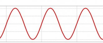
Unless you have a lot of experience with frequency domain analysis, you may be unsure of what these frequency components are and how they coexist in a signal that cannot have multiple voltage values at the same time. Let's look at a quick example to help clarify this concept.

Let's imagine that we have an audio signal that consists of a perfect 5 kHz sine wave. We know what a sine wave looks like in the time domain, but in the frequency domain we will see nothing but a frequency “spike” at 5 kHz. Now let's assume that we turn on a 500 kHz oscillator, which introduces high-frequency noise into the audio signal.

The signal seen on the oscilloscope will still be just one voltage train with one value at a time, but it will look different because its time domain variations should now reflect both the 5 kHz sine wave and the high frequency oscillations noise.

However, in the frequency domain, the sine wave and noise are separate frequency components that are present simultaneously in that one signal. A sine wave and noise occupy different parts of the frequency domain representation of a signal (as shown in the diagram below), and this means that we can filter out the noise by routing the signal through a circuit that allows low frequencies to pass through and blocks high frequencies.

Figure 3 – Frequency domain representation of audio signal and high-frequency noise

Russian Blogs

[Guide]: The previous article on IIR design, I still have a friend click on it to read. Although I don't know what the judges think, but thinking that there will always be a score, I decided to continue this series. In this article we will talk about the averaging filter, which at first glance is very simple. However, I personally believe that some key points may not be fully understood. This article focuses on the internal mechanism and application scenarios of the 1D mean xx filter design.

Note. Try to write annotations for each article for ease of reading. In the information age, everyone's time is valuable and this can also save fans' precious time.

To know one thing, personal advice should be based on three aspects: What Why How

The content here mainly refers to Section 7.5.1 "Introduction to Digital Signal Processing" compiled by Hu Guangshu with some insight of his own.

When it comes to averaging filters, friends who have been developing microcontroller applications may immediately think about adding and averaging some sample data. Indeed, this is also very intuitive from the mathematical description of the time domain: KaTeX parse error: No such environment: align* at position 8: \begin{̲a̲l̲i̲g̲n̲*̲}̲ y(n)&=\frac{1}… where x ( n ) x(n) x(n)Represents the current measured value. For SoC applications, this could be the current ADC sample value or a series of physical quantities processed by a current sensor (such as temperature, pressure, flow and other measured values in the industrial control field). x ( n − 1 ) x(n-1) x(n−1) Indicates the last measured value, etc. x ( n − N + 1 ) x(n-N+1) x(n−N+1 )This is the previous N-1 measurement value.

To reveal a deeper mechanism, the Z transfer function is used to further describe the above formula: KaTeX parse error: No such environment: align* at position 8: \begin{̲a̲l̲i̲g̲n̲*̲}̲ H(Z)&=\frac{1} … For the Fourier transform: X ( ω ) = ∑ k = − ∞ ∞ x ( n ) e − j ω n X(\omega)=\sum_{k=-\infty}^{\infty}x(n)e ^{-j\omega{n}} X(ω)=k=−∞∑∞x(n)e−jωn The essence of the Z-transform is a discrete form of the Laplace transform, Z = e σ + j ω = e σ ej ω Z=e^{\sigma+j\omega}=e^{\sigma}e^{j\omega} Z=eσ+jω=eσejω,do e σ = re^{\sigma}=r eσ= r,then X ( Z ) = ∑ k = − ∞ ∞ x ( n ) ( rej ω ) − n X(Z)=\sum_{k=-\infty}^{\infty}x(n)(re^ {j\omega})^{-n} X(Z)=k=−∞∑∞x(n)(rejω)−n Order r = 1 r=1 r=1,then X ( Z ） = ∑ k = − ∞ ∞ x ( n ) ej ω n X(Z）=\sum_{k=-\infty}^{\infty}x(n)e^{j\omega{n}} X(Z）= k=−∞∑∞x(n)ejωn Therefore, the frequency response of the average filter:

Use the following Python code for analysis

# encoding: UTF-8 from scipy.optimize import newton from scipy.signal import freqz, dimpulse, dstep from math import sin, cos, sqrt, pi import numpy as np import matplotlib.pyplot as plt import sys reload(sys) sys. setdefaultencoding('utf8') # The function is used to calculate the cutoff frequency of the moving average filter def get_filter_cutoff(N, **kwargs): func = lambda w: sin(N*w/2) — N/sqrt(2) * sin(w /2) deriv = lambda w: cos(N*w/2) * N/2 — N/sqrt(2) * cos(w/2) / 2 omega_0 = pi/N # Starting condition: halfway the first period of sin return newton(func, omega_0, deriv, **kwargs) # Set sample rate sample_rate = 200 #Hz N = 7 # Calculate cutoff frequency w_c = get_filter_cutoff(N) cutoff_freq = w_c * sample_rate / (2 * pi) # Filter parameters b = np.ones(N) a = np.array([N] + [0]*(N-1)) #Frequency response w, h = freqz(b, a, worN=4096) # Go to frequency w *= sample_rate / (2 * pi) # Draw a Bode plot plt.subplot(2, 1, 1) plt.suptitle("Bode") # Convert to decibels plt.plot(w, 20 * np.log10(abs(h ))) plt.ylabel('Magnitude [dB]') plt.xlim(0, sample_rate / 2) plt.ylim(-60, 10) plt.axvline(cutoff_freq, color='red') plt.axhline(- 3.01, linewidth=0.8, color='black', linestyle=':') # Phase frequency response plt.subplot(2, 1, 2) plt.plot(w, 180 * np.angle(h) / pi) plt .xlabel('Frequency [Hz]') plt.ylabel('Phase [°]') plt.xlim(0, sample_rate / 2) plt.ylim(-180, 90) plt.yticks([-180, -135 , -90, -45, 0, 45, 90]) plt.axvline(cutoff_freq, color='red') plt.show()

The sampling frequency is 200 Hz and the filter length is 7 to obtain the following amplitude-frequency and phase-frequency response curves. Its main lobe shows that its amplitude-frequency response is a low-pass filter. The amplitude-frequency response is slightly uneven and weakens with increasing frequency. Its phase frequency response is linear. Friends who have experience with filters know that the frequency-phase response of FIR filters is linear, and the moving average filter is just a special case of FIR filters.

When changing the filter length to 3/7/21, observe only its amplitude-frequency response:

You can see that as the filter length increases, its cutoff frequency becomes lower and the bandwidth becomes narrower. The filter response becomes slower and the latency increases. Therefore, in actual use, the filter length should be wisely selected according to the useful frequency band. The bandwidth of the desired signal can be obtained using Fourier analysis by collecting a specific point according to the sampling frequency. If you have an oscilloscope with FFT function, you can also measure it directly.

Implementing a filter in C is relatively simple. Here again the general code is used:

#define MVF_LENGTH 5 typedef float E_SAMPLE;
/ * Determine the historical state of the moving average register * / typedef struct _t_MAF { E_SAMPLE buffer[MVF_LENGTH]; E_SAMPLE sum; int index; }t_MAF; void moving_average_filter_init(t_MAF * pMaf) { pMaf->index = -1; pMaf->sum = 0; } E_SAMPLE moving_average_filter(t_MAF * pMaf,E_SAMPLE xn) { E_SAMPLE yn=0; int i=0; if(pMaf->index == -1) { for(i = 0; i < MVF_LENGTH; i++) { pMaf->buffer = xn;
} pMaf->sum = xn*MVF_LENGTH; pMaf->index = 0; } else { if(xn>100) xn = xn+0.1; pMaf->sum -= pMaf->buffer[pMaf->index]; pMaf->buffer[pMaf->index] = xn; pMaf->sum += xn; pMaf->index++; if(pMaf->index>=MVF_LENGTH) pMaf->index = 0; } yn = pMaf->sum/MVF_LENGTH; return yn; } Test code:

#define SAMPLE_RATE 500.0f #define SAMPLE_SIZE 256 #define PI 3.415926f int main() { E_SAMPLE rawSin[SAMPLE_SIZE];
E_SAMPLE outSin[SAMPLE_SIZE]; E_SAMPLE rawSquare[SAMPLE_SIZE]; E_SAMPLE outSquare[SAMPLE_SIZE]; t_MAF mvf; FILE *pFile=fopen(“./simulationSin.csv”,”wt+”); / * Square wave test * / if(pFile==NULL) { printf("simulationSin.csv opened failed"); return -1; } for(int i=0;i = 100*sin(2*PI*20*i/SAMPLE_RATE)+rand()%30;
} / * Sine wave test * / for(int i=0;i For the square wave test, use Excel to generate the waveform and the following waveform can be obtained. From the waveform, it is obvious that a moving average filter with a length of 7 is relatively satisfactory for the random noise filtering effect. The figure also shows that the moving average filter introduces a certain delay into the signal chain, which must be taken into account when using it. If there are no clear requirements for the overall sensor measurement, it can often be ignored.

For sine wave signals, the moving average filter also has a more obvious effect, but its bandwidth is relatively narrow. If the frequency of the desired signal is relatively high, a moving average filter is not suitable.

to sum up:

The moving average filter works well at filtering out high frequency noise.
A moving average filter is essentially an FIR filter with a linear phase frequency response.
In practical use, pay attention to the frequency of the wanted signal, if the frequency of the wanted signal is higher, it is not applicable.
The length should not be too long, otherwise the delay effect will be large.
From a signal chain point of view, it can be used as pre-processing, that is, data after direct filtering by the ADC. It can also be used as post-processing.
If it is filtering ADC sample data, the sample is integer, the code in the text can be optimized accordingly, for example, multiplication and division can be replaced by left shift and right shift.

Copyright Statement: All articles are copyrighted by Built-in Hotel, for example, commercial use must be permitted by Built-in Hotel. We invite you to subscribe to the official WeChat account, the content is richer.

Filter order and quality factor

The next parameter that you need to decide on is the order of the filter and its quality factor. This article will consider two orders, first and second.

With the first, everything is simple: there is a coil, there is a capacitor, we calculate their parameters for the required cutoff frequency and, if necessary, adjust the values until the desired frequency response, phase response, and frequency response are obtained.
The second order is trickier, there are already two coils and two capacitors. A parameter such as the quality factor depends on the values of the nominal values; it determines the steepness of the frequency response decline and, to some extent, the phase shift. Since the influence of the phase shift and slope cannot be speculatively estimated, all that remains is to simply choose which way to think. And think here in the direction of low quality factor, read more inductance in the coils, less capacitance in the capacitors.

How to choose an order. Here we are guided by already familiar considerations about what emitters, especially high-frequency speakers, are capable of. If a big move is contraindicated for him (as in our case), then we give preference to the second order.

To complete the picture, it should be mentioned that the order also determines the degree to which the speakers work together, but this is information for independent reflection.

Filters. Phase and its derivative

Now that we have accumulated a certain amount of material, we can move on to the phase. It must be said from the very beginning that the concept of phase was introduced a long time ago to serve the needs of electrical engineering.

When the signal is a pure sine (although the degree of purity varies) of a fixed frequency, then it is quite natural to represent it in the form of a rotating vector, determined, as is known, by the amplitude (modulus) and phase (argument). For an audio signal, in which the sines are present only in the form of decomposition, the concept of phase is no longer so clear. However, it is no less useful - if only because sound waves from different sources are added vectorially. Now let's see what the phase-frequency characteristics (PFC) of filters up to the fourth order inclusive look like. The numbering of the figures will remain continuous, from the previous issue.

We begin, therefore, with Fig. 12 and 13.

rice. 12

rice. 13

You can immediately notice interesting patterns.

1. Any filter “twists” the phase by an angle that is a multiple of π/4, more precisely, by an amount (nπ)/4, where n is the order of the filter.

2. The phase response of the low-pass filter always starts from 0 degrees.

3. The phase response of the high-pass filter always comes at 360 degrees.

The last point can be clarified: the “destination point” of the phase response of the high-pass filter is a multiple of 360 degrees; if the filter order is higher than the fourth, then with increasing frequency the phase of the high-frequency filter will tend to 720 degrees, that is, 4π, if higher than the eighth - to 6π, etc. But for us this is pure mathematics, which has a very distant relationship to practice.

From a joint consideration of the listed three points, it is easy to conclude that the phase response characteristics of the high-pass and low-pass filters coincide only for the fourth, eighth, etc. orders, and the validity of this statement for fourth-order filters is clearly confirmed by the graph in Fig. 13. However, it does not follow from this fact that the fourth-order filter is “the best”, just as, by the way, the opposite does not follow. In general, it’s too early to draw conclusions.

The phase characteristics of filters do not depend on the implementation method - they are active or passive, and even on the physical nature of the filter. Therefore, we will not specifically focus on the phase response characteristics of passive filters; for the most part, they are no different from those that we have already seen. By the way, filters are among the so-called minimum-phase circuits - their amplitude-frequency and phase-frequency characteristics are strictly interconnected. Non-minimum phase links include, for example, a delay line.

It is quite obvious (if there are graphs) that the higher the order of the filter, the steeper its phase response drops. How is the steepness of any function characterized? Its derivative. The derivative of the phase response with respect to frequency has a special name - group delay time (GDT). The phase must be taken in radians, and the frequency must be taken not as vibrational (in hertz), but as angular, in radians per second. Then the derivative will receive the dimension of time, which explains (albeit partially) its name. The group delay characteristics of high-pass and low-pass filters of the same type are no different. This is what the group delay graphs look like for Butterworth filters from the first to the fourth order (Fig. 14).

rice. 14

Here the difference between filters of different orders seems especially noticeable. The maximum (in amplitude) group delay value for a fourth-order filter is approximately four times greater than that of a first-order filter and twice that of a second-order filter. There are statements that according to this parameter, a fourth-order filter is just four times worse than a first-order filter. For a high pass filter it is possible. But for a low-pass filter, the disadvantages of a high group delay are not so significant in comparison with the advantages of a high frequency response slope.

For further discussion, it will be useful for us to imagine what the phase response “over the air” of an electrodynamic head looks like, that is, how the radiation phase depends on frequency.

rice. 15

A remarkable picture (Fig. 15): at first glance it looks like a filter, but, on the other hand, it is not a filter at all - the phase drops all the time, and with an increasing steepness. I won’t let on any unnecessary mystery: this is what the delay line phase response looks like. Experienced people will say: of course, the delay is caused by the travel of the sound wave from the emitter to the microphone. And experienced people will make a mistake: my microphone was installed along the head flange; Even if we take into account the position of the so-called center of radiation, this can cause an error of 3 - 4 cm (for this particular head). And here, if you estimate, the delay is almost half a meter. And, in fact, why shouldn’t there be a delay? Just imagine such a signal at the output of the amplifier: nothing, nothing, and suddenly a sine - as it should be, from the origin and with maximum slope. (For example, I don’t need to imagine anything, I have this written down on one of the measuring CDs, we check the polarity using this signal.) It is clear that the current will not flow through the voice coil immediately, it still has some kind of inductance. But these are minor things. The main thing is that sound pressure is volumetric velocity, that is, the diffuser must first accelerate, and only then sound will appear. For the delay value, it is probably possible to derive a formula; it will probably include the mass of the “movement”, the force factor and, possibly, the ohmic resistance of the coil. By the way, I obtained similar results on different equipment: both on the Bruel & Kjaer analog phase meter, and on the MLSSA and Clio digital complexes. I know for sure that mid-frequency drivers have less delay than bass drivers, and tweeters have less delay than both of them. Surprisingly, I have not seen any references to such results in the literature.

Why did I bring this instructive graph? And then, if this is really the case as I see it, then many discussions about the properties of filters lose practical meaning. Although I will still present them, and you can decide for yourself whether all of them are worth adopting.

Passive filter circuits

I think few people will be surprised if I say that there are much fewer circuit implementations of passive filters than active filters. I would say there are about two and a half. That is, if elliptic filters are put into a separate class of circuits, you get three, if you don’t do this, then two. Moreover, in 90% of cases in acoustics, so-called parallel filters are used. Therefore, we will not start with them.

Serial filters, unlike parallel ones, do not exist “in parts” - here is a low-pass filter, and there is a high-pass filter. This means you cannot connect them to different amplifiers. In addition, in terms of their characteristics, these are first-order filters. And by the way, the ubiquitous Mr. Small substantiated that first-order filters are unsuitable for acoustic applications, no matter what orthodox audiophiles (on the one hand) and supporters of every possible reduction in the cost of acoustic products (on the other) say. However, series filters have one advantage: the sum of their output voltages is always equal to unity. This is what the circuit of a two-band sequential filter looks like (Fig. 16).

rice. 16

In this case, the values correspond to a cutoff frequency of 2000 Hz. It is easy to understand that the sum of the voltages across the loads is always exactly equal to the input voltage. This feature of the serial filter is used when “preparing” signals for further processing by the processor (in particular, in Dolby Pro Logic). In the next graph you see the frequency response of the filter (Fig. 17).

rice. 17

You can believe that its phase response and group delay graphs are exactly the same as those of any first-order filter. A three-band sequential filter is also known to science. Its diagram is in Fig. 18.

rice. 18

The values shown in the diagram correspond to the same crossover frequency (2000 Hz) between the tweeter (HF) and the midrange driver and the frequency of 100 Hz - the crossover frequency between the midrange and low-frequency heads. It is clear that a three-band series filter has the same property: the sum of the voltages at its output is exactly equal to the voltage at the input. In the following figure (Fig. 19), which shows a set of characteristics of this filter, you can see that the slope of the tweeter filter roll-off in the range 50 - 200 Hz is higher than 6 dB/oct., since its band here overlaps not only with the midrange band , but also to the woofer head band. This is what parallel filters cannot do - their overlap of bands inevitably brings surprises, and always unpleasant ones.

rice. 19

The parameters of the sequential filter are calculated in exactly the same way as the values of the first order filters. The dependence is still the same (see formula 1.1). It is most convenient to introduce the so-called time constant; through the filter cutoff frequency it is expressed as TO = 1/(2πFc).

Then

C = TO/RL (2.1), and

L = TO • RL (2.2).

(Here RL is the load impedance, in this case 4 ohms).

If, as in the second case, you have a three-band filter, then there will be two crossover frequencies and two time constants.

Probably, the most technically savvy of you have already noticed that I slightly “distorted” the cards and replaced the real load impedance (that is, the speaker) with an ohmic “equivalent” of 4 Ohms. In reality, of course, there is no equivalent. In fact, even a forcibly inhibited voice coil, from the point of view of an impedance meter, looks like active and inductive reactance connected in series. And when the coil is mobile, the inductance increases at a high frequency, and near the resonance frequency of the head, its ohmic resistance seems to increase, sometimes ten times or more. There are very few programs that can take into account such features of a real head; I personally know of three. But we in no way set out to learn how to work in, say, the Linearx software environment. Our task is different - to understand the main features of filters. Therefore, we will, in the old fashioned way, simulate the presence of a head with a resistive equivalent, and specifically with a nominal value of 4 Ohms. If in your case the load has a different impedance, then all the impedances included in the passive filter circuit must be proportionally changed. That is, inductance is proportional, and capacitance is inversely proportional to the load resistance.

(After reading this in a draft, the editor-in-chief said: “What, sequential filters are the Klondike, let’s dig into it somehow.” I agree. Klondike. I had to promise that we’ll dig into it separately and specifically in one of the upcoming issues.)

The most widely used parallel filters are also called “ladder” filters. I think it will be clear to everyone where this name comes from after you look at the generalized filter circuit (Fig. 20).

rice. 20

To get a fourth-order low-pass filter, you need to replace all horizontal “bars” in this circuit with inductances, and all vertical ones with capacitors. Accordingly, to build a high-pass filter you need to do the opposite. Lower order filters are obtained by discarding one or more elements, starting with the last one. Higher order filters are obtained in a similar way, only by increasing the number of elements. But we will agree: there are no filters higher than the fourth order for us. As we will see later, along with the increase in filter steepness, their shortcomings also deepen, so such an agreement is not something seditious. To complete the presentation, it would be necessary to say one more thing. There is an alternative option for constructing passive filters, where the first element is always a resistor rather than a reactive element. Such circuits are used when it is necessary to normalize the input impedance of the filter (for example, operational amplifiers “do not like” loads less than 50 Ohms). But in our case, an extra resistor means unjustified power losses, so “our” filters begin with reactivity. Unless, of course, you need to specifically reduce the signal level.

The most complex bandpass filter in design is obtained if in a generalized circuit each horizontal element is replaced with a series connection of capacitance and inductance (in any sequence), and each vertical element must be replaced with a parallel connection - also capacitance and inductance. Probably, I will still give such a “scary” diagram (Fig. 21).

rice. 21

There is one more little trick. If you need an asymmetrical “bandpass” (bandpass filter), in which, say, the high-pass filter is of the fourth order, and the low-pass filter is of the second, then the unnecessary parts from the above circuit (that is, one capacitor and one coil) must definitely be removed from “ tail" of the circuit, and not vice versa. Otherwise, you will get somewhat unexpected effects from changing the nature of the loading of the previous filter cascades.

We did not have time to get acquainted with elliptical filters. Well, then, next time we’ll start with them.

Tags: PhaseFilters

Cutoff frequency

The range of frequencies for which the filter does not cause significant attenuation is called the passband, and the range of frequencies for which the filter causes significant attenuation is called the stopband. Analog filters, such as the RC low-pass filter, always transition from passband to stopband gradually. This means that it is impossible to identify a single frequency at which the filter stops passing signals and begins to block them. However, engineers need a way to conveniently and concisely characterize the frequency response of a filter, and this is where the concept of cutoff frequency comes into play.

When you look at the frequency response graph of an RC filter, you will notice that the term “cutoff frequency” is not very accurate. A picture of the spectrum of a signal being "cut" into two halves, one of which is retained and the other discarded, is not applicable because the attenuation increases gradually as frequencies move from values below the cutoff frequency to values above the cutoff frequency.

The cutoff frequency of an RC low-pass filter is actually the frequency at which the amplitude of the input signal is reduced by 3 dB (this value was chosen because a 3 dB reduction in amplitude corresponds to a 50% reduction in power). Thus, the cutoff frequency is also called the -3 dB frequency, and this name is actually more accurate and more descriptive. The term bandwidth refers to the bandwidth of the filter, and in the case of a low-pass filter, the bandwidth is equal to the frequency -3 dB (as shown in the diagram below).

Figure 8 – This diagram shows the general features of the amplitude-frequency response of an RC low-pass filter. The bandwidth is equal to the frequency -3 dB.

As explained above, the low-pass pass behavior of an RC filter is due to the interaction between the frequency-independent impedance of the resistor and the frequency-dependent impedance of the capacitor. To determine the details of a filter's frequency response, we need to mathematically analyze the relationship between resistance (R) and capacitance (C); we can also manipulate these values to design a filter that meets precise specifications. The cutoff frequency (fcf) of the RC low pass filter is calculated as follows:

Let's look at a simple example. Capacitor values are more restrictive than resistor values, so we'll start with a common capacitance value (such as 10 nF) and then use a formula to determine the required resistance value. The goal is to design a filter that will preserve the 5 kHz audio signal and reject the 500 kHz noise. We'll try a cutoff frequency of 100 kHz, and later in this article we'll analyze the effect of this filter on both frequency components more closely.

Thus, a 160 Ohm resistor in combination with a 10 nF capacitor will give us a filter that gives a frequency response close to the required one.

Operational amplifiers (based on simple examples): part 3

Brief introduction

I continue to write spam on the topic of operational amplifiers. In this article I will try to give an overview of one of the most important topics related to op amps. So, welcome, active filters
.

Topic overview

You may have already come across RC, LC and RLC filter models. They are quite suitable for most tasks. But for some applications, it is very important to have filters with flatter bandwidth characteristics and steeper slopes. This is where we need active filters. To refresh your memory, let me remind you what filters are: Low Pass Filter (LPF) - passes a signal that is below a certain frequency (also called the cutoff frequency). Wikipedia High Pass Filter (HPF) - passes a signal above the cutoff frequency. Wikipedia Bandpass Filter - passes only a certain range of frequencies. Wikipedia Notch Filter - blocks only a certain range of frequencies. Wikipedia Well, a little more poetry. Look at the amplitude-frequency response (AFC) of the high-pass filter. Don’t look for anything interesting on this graph yet, but just pay attention to the sections and their names: The most common examples of active filters can be seen here in the “Integrators and differentiators” section. But in this article we will not touch these circuits, because they are not very effective.

Selecting a filter

Let's assume that you have already decided on the frequency you want to filter. Now you need to decide on the type of filter. More precisely, you need to choose its characteristics. In other words, how the filter will “behave.” The main characteristics are: Butterward filter
- has the flattest response in the passband, but has a smooth roll-off.
Chebyshev filter
- has the steepest roll-off, but it has the most uneven characteristics in the passband.
Bessel filter
- has a good phase-frequency response and quite a “decent” roll-off. Considered the best choice if there is no specific task.

Some more information

Let's assume you completed this task.
And now you can safely begin the calculations. There are several calculation methods. Let's not complicate things and use the simplest. And the simplest one is the “tabular” method. Tables can be found in the relevant literature. So that you don’t have to search for a long time, I will quote from Horowitz and Hill “The Art of Circuit Design”. For the low-pass filter: Let's just say that you could find and read all this in literature. Let's move on specifically to filter design.

Calculation

In this section I will try to briefly go over all types of filters. So, task #1
.
Construct a second-order low-pass filter with a cutoff frequency of 150 Hz according to the Butterward characteristic. Let's get started. If we have a filter of the nth even order, this means that it will have n/2 opamps. In this task - one. Low-pass filter circuit: For this type of calculation, it is taken into account that R1 = R2
,
C1 = C2
.
Let's look at the sign. We see that K = 1.586
.
We'll need this a little later. For a low-pass filter, the following is true: , where, of course, is the cutoff frequency. Having done the calculation, we get . Now let's start selecting the elements. We decided on the op-amp - “ideal” in the amount of 1 piece. From the previous equality we can assume that it does not matter to us which element we choose “first”. Let's start with the resistor. It is best that its resistance value be in the range from 2 kOhm to 500 kOhm. By eye, let it be 11 kOhm. Accordingly, the capacitance of the capacitor will become equal to 0.1 µF. For feedback resistors, we take the value of R
arbitrarily.
I usually take 10 kOhm. Then, for the upper value we take K from the table. Therefore, the lower one will have a resistance value of R =
10 kOhm, and the upper one will have a resistance value of 5.8 kOhm. Let's collect and simulate the frequency response.

Task #2

.
Construct a fourth-order high-pass filter with a cutoff frequency of 800 Hz using the Bessel characteristic. Let's decide. Since it is a fourth-order filter, there will be two op-amps in the circuit. Everything here is not difficult at all. We simply cascade 2 high-pass filter circuits. The filter itself looks like this: A fourth-order filter looks like this: Now the calculation. As you can see, for a fourth-order filter we have as many as 2 K
.
It is logical that the first is intended for the first cascade, the second - for the second. The K
values are 1.432 and 1.606, respectively.
The table was for low-pass filters (!). To calculate the high-pass filter, you need to change something. K
coefficients remain the same in any case.
For the Bessel and Chebyshev characteristics, the parameter—the normalizing frequency—changes. It will now be equal to: For Chebyshev and Bessel filters, both for low frequencies and for high frequencies, the same formula is valid: Please note that for each individual cascade you will have to count separately. For the first stage: Let C
= 0.01 µF, then
R
= 28.5 kOhm.
Feedback resistors: lower, as usual, 10 kOhm; upper - 840 Ohms. For the second stage: Leave the capacitance of the capacitor unchanged. Since C =
0.01 µF, then
R
= 32 kOhm. We are building the frequency response.

To create bandpass or notch filters, you can cascade a low-pass filter and a high-pass filter. But these types are often not used due to poor characteristics. For bandpass and notch filters, you can also use the “table method”, but the characteristics are slightly different. I’ll just give you a sign and explain it a little. In order not to stretch it too much, the values were taken immediately for a fourth-order bandpass filter. a1

and
b1
are the calculated coefficients.
Q
- quality factor.
This is a new option. The higher the value of the quality factor, the more “sharp” the decline will be. Δf
is the range of transmitted frequencies, and the sampling is at a level of -3 dB.
Coefficient α
is another calculated coefficient.
It can be found using formulas that are quite easy to find on the Internet. Okay, that's enough. Now the work task. Task #3
.
Construct a fourth-order bandpass filter using the Butterward characteristic with a center frequency of 10 kHz, a bandwidth of transmitted frequencies of 1 kHz, and a gain at the center frequency point equal to 1. Let's go. Fourth order filter. That means two op-amps. I’ll give you a typical diagram with calculation elements right away. For the first filter, the central frequency is determined as: For the second filter: Specifically in our case, again from the table, we determine that the quality factor is Q
= 10. We calculate the quality factor for the filter.
Moreover, it is worth noting that the quality factor of both will be equal. Gain correction for the center frequency region: The final stage is the calculation of the components. Let the capacitor be 10 nF. Then, for the first filter: In the same order as (1) we find R22 = R5 =
43.5 kOhm,
R12 = R4
= 15.4 kOhm,
R32 = R6
= 54.2 Ohm. Just keep in mind that for the second filter we use And lastly, frequency response.

The next stop is band-stop or notch filters. There are several variations here. Probably the simplest is the Wien-Robinson Filter. The typical circuit is also a 4th order filter. Our last task. Task #4

.
Construct a notch filter with a central frequency of 90 Hz, quality factor Q
= 2 and gain in the passband equal to 1. First of all, we randomly select the capacitance of the capacitor.
Let's say C =
100 nF.
Let's determine the value R6 = R7 = R
: It is logical that by “playing” with these resistors, we can change the frequency range of our filter.
Next, we need to determine intermediate coefficients. We find them through quality factor. Let's choose resistor R2
.
In this particular case, it is best for it to be 30 kOhm. Now we can find resistors that will regulate the gain in the passband. And finally, you need to arbitrarily choose R5 = 2R1
. In my circuit, these resistors have a value of 40 kOhm and 20 kOhm, respectively. Actually, frequency response:

Almost the end

For those interested in learning a little more, I can recommend reading Horowitz and Hill’s “The Art of Circuit Design.” Also, D. Johnson “A handbook of active filters”. Wikipedia Also, for those who don’t really need calculations, but just need the filters themselves, I can recommend useful software PS I’ll add a very useful link and its mirror. Thanks for the link spiritus_sancti

Flattening filters

Now the final stage begins - mixing the filters. It's time to wind the reels... or not to wind them? You are always too lazy to wind, there are no wires, frames, or specific inductance values. In view of these reasons, after searching in the trash, we found pairs of 0.8 mcg and 3 mcg coils - we had to build on them. In extreme cases, you can always rewind or unwind the excess.

The graph shows that the section fell into the region of 1.8 kHz, which fits well within the intended boundaries. By selecting capacitors we managed to achieve the following impedance. There are two bumps at the crossover frequency, but their height is less than half an ohm - this is not critical. This is not its final form; subsequently the resistor in the Zobel circuit of the tweeter was slightly increased.

The above pictures show the frequency response of both the filter itself and the frequency response of the speakers with it turned on.

Speaker impedance characteristic

When everything is more or less clear with the approximate parameters, it’s time to move on to practice. We take the impedance characteristics of the speakers. In order to estimate the resistance, the graph has a ladder in steps of one ohm. A jump at 110 hertz is a switch from 10 ohms to 20.

Of course, with such humps, not a single filter will work normally, and especially not a low-pass filter. In general, this rise does not interfere with the work of the high-pass filter, however, as mentioned earlier, such a rise at the end of the range will lead to a rise in high frequencies if the amplifier has a high resistance. This can also be used for good, leaving the rise small.

For an approximate idea of what depends on what, I provide a set of graphs for various capacitances and resistances. The step starts at 10 ohms.

Knowing the minimum resistance of the low-frequency link, you need to bring the high-frequency link to the same.
There are many options for how to connect two resistors and a Zobel chain, and anyone who has decided to take such a brave step as mixing is able to determine the type of connection and resistor values, so it is unnecessary to describe this procedure here. Specifically, in these speakers, based on the results of preliminary listening, it was decided to leave the original 2.2 ohm resistors and the Zobel circuit parallel to the tweeter. No tags for this post.

Minimal impact on phase response

The amplitude-frequency response (AFC) of the Bessel (aka Thompson) filter is linear throughout the entire passband. But its main advantage is the absence of introduced phase distortions. Those. For all frequencies in the passband the delay is the same.

In terms of phase response, it is ideal for use in audio circuits. But its fly in the ointment is the gentlest decline among all filters. RC circuit has a more gradual decline .

The following figure compares the slopes of filter cuts of different types: 1 - Bessel, 2 - Butterworth, 3 - Chebyshev (unevenness 0.5 dB).

The Butterworth filter has similar characteristics to the Bessel filter, but it has a steeper frequency response rolloff. You have to pay for this by the unevenness of the delay for different frequencies.

The dependence of the signal delay time on frequencies for Bessel (1) and Butterward (2) filters of the second order, normalized by frequency, is shown in the following figure:

Please note that the graph shows cyclic frequency (omega). To convert to hertz, you need to multiply it by 2π. In addition, a linear rather than logarithmic scale is used along the X-axis.

But still, the Butterward filter is not so bad. Although I wouldn't recommend using it in audio circuits. Or you should choose a higher cutoff frequency so that phase distortion in the desired range is minimal. But in practice this is not always possible.