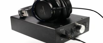
An op-amp headphone amplifier circuit that definitely deserves attention. For all its simplicity, such a headphone amplifier will rock any headphones. And the main feature is the doubled output current compared to conventional op-amp switching.
UPD[04/24/2020] - the article was heavily rewritten, and the diagram was changed, so some comments are no longer relevant.
My amplifier assembly video:
Headphone amplifier circuit
Wandering through the vast expanses of the trash heap of knowledge - the Internet - led to an interesting discovery. It was a PDF from Burr Brown. The find inspired me to build an op-amp headphone amplifier.
From the language of a potential enemy, the file name can be literally translated as follows: Doubling the output current to the load with two audio op-amps OPA2604 . You can download this PDF using a direct link from my website.
download: Double the output current to a load with the dual OPA2604 audio op amp
The file consists of two pages, where only the first is valuable. The headphone amplifier circuit presented there was redrawn and got rid of unnecessary clever inscriptions.
Meet this future heart of our amplifier. To be more precise, this is a diagram of one channel.
We will have 2 channels and each needs 2 op-amps. The most convenient option would be to use dual operational amplifiers.
Resistors R3 and R4 with a resistance of 51 Ohms are needed to protect the outputs of the operational amplifiers by current.
A little history
In the 40s of the twentieth century, due to the rapid development of science and technology, a need arose for devices that would allow high-speed calculations and perform basic mathematical operations such as addition, multiplication, exponentiation, logarithm, differentiation, integration and etc. Such a device was called an operational amplifier, and it was based on the differential amplifier, which we discussed in the previous article. Since many operational amplifiers were used for computing tasks, such devices were called analog computers (AVMs) or analog computers.
The production of analog computers peaked in the 1960-1970s and they were used in all areas of science and technology, but over time they were replaced by digital computing devices. However, with the advent of the era of digital devices and computers, the relevance of operational amplifiers has not lost its importance. Although their “operational” functions have faded into the background, the operational amplifier, being in its essence an almost ideal amplifier, has the same importance in analog technology as a logic inverter, which performs the simplest logical function, in digital technology.
The first operational amplifiers were made on the basis of vacuum tubes and had the size of a brick (developed in the 40-50s) with rather modest parameters. Modern operational amplifiers, made using integrated technology of the latest generations, have a frequency band from 5 kHz to 5 GHz, and the supply voltage ranges from 0.9 V to 1000 V.
What is the “trick” of this amplifier?
The scheme is not new at all. It is known from datasheets of the 90s. But the interesting thing about the circuit is that both op-amps amplify the same signal. But this is not a bridge connection. The output signals of both op-amps are in phase, due to which their output currents add up.
This inclusion solves the problem of the low output current of many op-amps. This significantly increases the number of op amps that can be used in the amplifier. Now it is enough that each operational amplifier can provide an output current of 35-40 mA, instead of 70-80 in the case of one op-amp per channel.
The maximum output current value is always given in the datasheets on the op-amp.
Gain
The resulting circuit is a non-inverting amplifier. The signal amplification factor is determined by resistors R1 and R2 . Its exact value is determined by the formula:
K= 1+ R2/R1
We will assume that we are applying a signal from the linear output to the input. In this case, the stress force coefficient equal to 3 will be with a good margin. Therefore, we will be equal to three.
The accuracy of resistors R1 and R2 determines how equal the gain of the channels will be. Therefore, it is desirable that resistors have an accuracy of no worse than ±1% . It is not always possible to find a large assortment of resistor values with good accuracy in stores or in home supplies. But in this case, you can get by with resistors of the same value.
So, in the bins of the cabinet, precision resistors of 7.5 kOhm were found, which became resistors R1 . As R2, two 7.5 kOhm resistors were used, which were connected in series. You can do the same thing by connecting in parallel two 15 kOhm resistors as R1 , and one 15 kOhm resistor as R2 .
To change the gain, it is better to change the resistor R2 . For op-amp audio circuits, it is usually recommended to use resistors with a nominal value of 1÷50 kOhm. Any resistor introduces noise into the audio path, and the higher the value of this resistor, the greater the noise it introduces.
What will happen at the output of the op-amp if there are zero volts at both inputs?
So, we have considered the case when the voltage at the inputs may differ. But what happens if they are equal? What will Proteus show us in this case? Hmm, showed +Upit.
What will Falstad show? Zero Volt.
Who to believe? No one! In real life, it is impossible to do this in order to drive absolutely equal voltages to the two inputs. Therefore, such a state of the op-amp will be unstable and the output values can take values of either -E Volt or +E Volt.
Let's apply a sinusoidal signal with an amplitude of 1 Volt and a frequency of 1 kilohertz to the non-inverting input, and put the inverting one to ground, that is, to zero.
Let's see what we have on the virtual oscilloscope:
What can be said in this case? When the sinusoidal signal is in the negative region, we have -Upit at the output of the op-amp, and when the sinusoidal signal is in the positive region, then we have +Upit at the output.
Let's finalize the scheme
The diagram presented in the document is somewhat incomplete. For normal operation, the circuit should be supplemented with input circuits.
Operational amplifiers are equally good at amplifying both AC and DC voltages. Therefore, despite all sorts of audiophile troubles, it is considered good form to add a capacitor to the input.
Of course, modern sources do not provide a constant voltage to the output, but I don’t know where you will connect the amplifier... and I’m not eager to be responsible for your burned-out headphones
In addition to the capacitor that cuts off the DC voltage, you should add a resistor going to ground. Such a resistor will ensure that the non-inverting input of the op-amp is tied to ground. On the other side. together with the capacitor it forms an RC differentiating circuit.
The resulting RC circuit ( R5 , C1 ) will cut off both DC voltage and infra-low frequencies. They do not carry useful information, but they significantly load the amplifier with current. At the ratings indicated in the diagram, the cutoff frequency is 16 Hz. When using a 220nF capacitor, the cutoff frequency will drop to approximately 7Hz. Further increase in capacity does not make much sense.
To exclude possible self-excitation of the op-amp, it would not be amiss to limit the upper range. To do this, install a small capacitor R2
Circuit R2 C2 will act as a low pass filter. With the specified part ratings, the cutoff frequency will be about 100 kHz.
Operational Amplifiers: 10 Circuits for (Almost) Every Occasion
Hi all! Recently, I have mostly gone into digital and, partly, into power electronics and rarely use operational amplifier circuits. In this regard, obeying the steady law of memory half-life, my knowledge about operational amplifiers began to gradually fade, and every time I still needed to use this or that circuit with their participation, I had to Google its calculation or look for it in books. This turned out to be not very convenient, so I decided to write a kind of cheat sheet in which I reflected the most commonly used circuits on operational amplifiers, giving their calculations, as well as simulation results in LTSpice.
Introduction
This article will look at ten commonly used operational amplifier circuits.
When writing this article, I assumed that the reader knows what an operational amplifier is and at least has a general understanding of how it works. It is also assumed that he knows basic electrical circuit theory, such as Ohm's law or voltage divider calculations. This article should not be taken as a complete guide to using op amps in any situation. For a large number of tasks, indeed, these schemes may be sufficient, but in complex projects something non-standard may always be required.
Non-inverting amplifier
A non-inverting amplifier is probably the most common operational amplifier circuit; it is shown in the figure below.
In this circuit, the amplified signal is fed to the non-inverting input of the operational amplifier, and the output signal is fed through a voltage divider to the inverting input. The calculation of this circuit is simple, it is based on the fact that the operational amplifier, covered by a feedback loop, processes the input effect in such a way that the voltage at the inverting input is equal to the voltage at the non-inverting input: From this formula, the gain of the non-inverting amplifier is easily obtained: Let's calculate and simulate non-inverting amplifier with the following parameters:
- Operational amplifier LT1803
- Gain
- Input frequency
- Input amplitude
- DC component of the input signal
Let's choose from the range E96 and. Then the gain will be equal to The result of modeling this circuit is shown in the figure (picture clickable):
Let's now look at the edge cases of this amplifier.
Let's say the value of the resistor is . In this case, we find that the gain will tend to infinity. In fact, of course, although this is a very large, it is still a finite value; it is usually given in the documentation for the chip of a specific operational amplifier. On the other hand, the output voltage of a real operational amplifier, even with an infinitely large gain, cannot be infinitely large: it is limited by the supply voltage of the microcircuit. In practice, it is often even somewhat less, with the exception of some types of amplifiers that are marked as rail-to-rail. But in any case, it is not recommended to drive operational amplifiers to their limiting states: this leads to saturation of their internal output stages, nonlinear distortions and overloads of the microcircuit. Therefore, this limiting case does not have any practical benefit. Of much greater interest is another limiting case, when the resistance value is . We will look at it in the next section.
Repeater
As mentioned earlier, turning on an operational amplifier in a repeater circuit is the limiting case of a non-inverting amplifier, when one of the resistors has zero resistance. The repeater circuit is shown in the figure below.
As can be seen from the formula given in the last section, the transmission coefficient for a repeater is equal to one, that is, the output signal exactly repeats the input signal. Why do you need an operational amplifier in this case? It acts as a buffer, having a high input impedance and a low output impedance. When is this necessary? Let's say we have some kind of signal source with a high output impedance and want to transmit this signal without distortion to a relatively low-impedance discharge. If we do this directly, without any buffers, we will inevitably lose some part of the signal.
Let's verify this by simulating a circuit with the following main parameters:
- Signal source output impedance 10 kOhm
- Load resistance 1 kOhm
- Input frequency
- Input amplitude
- DC component of the input signal
We will carry out simulations for two cases: in the first case, let the signal source operate to the load through a repeater, and in the second case, directly. The simulation results are shown in the figure below (the picture is clickable): on the top oscillogram, the output and input signals exactly coincide with each other, while on the bottom, the output signal is several times smaller in amplitude relative to the input signal.
Instead of a follower on an operational amplifier, you can also use an emitter follower on a transistor, without forgetting, however, about its inherent limitations.
Inverting amplifier (classical circuit)
In the inverting amplifier circuit, the input signal is supplied to the inverting pin of the microcircuit, and feedback is also connected to it. The non-inverting input is connected to ground (sometimes to a bias source). A typical inverting amplifier circuit is shown in the figure below.
For the input circuit of the inverting amplifier, you can write the following expression: Where is the voltage at the inverting input of the operational amplifier. Since the operational amplifier, covered by a feedback loop, strives to equalize the voltages at its inputs, then, and with a grounded non-inverting input, we obtain. Hence, the gain of the inverting amplifier is equal. For the inverting amplifier, the following conclusions can be drawn:
- An inverting amplifier inverts the signal. This means that it is necessary to use bipolar power.
- The magnitude of the gain of the inverting amplifier is equal to the ratio of the feedback circuit resistors. If the values of two resistors are equal, the gain is -1, i.e. An inverting amplifier simply works as a signal inverter.
- The value of the input resistance of the inverting amplifier is equal to the value of resistor R1. This is important because with small values of R1 the previous stage can be heavily loaded.
For example, let's calculate an inverting amplifier with the following parameters:
- Operational amplifier LT1803
- Gain
- Input frequency
- Input amplitude
- DC component of the input signal
As resistors in the feedback circuit, we will choose resistors with nominal values and: their ratio is exactly equal to ten. The results of amplifier modeling are shown in the figure (picture clickable).
As you can see, the output signal is 10 times larger in amplitude than the input signal, and at the same time it is inverted.
The input impedance of this circuit is . What will happen if the signal source has a significant output impedance, say the same 10 kOhm? The result of modeling this case is presented in the figure below (the picture is clickable).
The amplitude of the output signal dropped by half compared to the previous case! Obviously, this is all due to the fact that the output impedance of the generator in this case is equal to the input impedance of the inverting amplifier. Thus, it is worth always remembering this feature of the inverting amplifier. What to do if you still need to ensure the operation of a signal source with a high output impedance to an inverting amplifier? In theory, you need to increase the resistance R1. However, at the same time, resistance R2 will also increase. If we want to provide a circuit input impedance of 500 kΩ at a gain of 10, resistor R2 must have a resistance of 5 MΩ! It is not recommended to use such large resistance values: the circuit will be very sensitive to interference, dust and flux on the printed circuit board. Are there any ways out of this situation? Actually yes. You can, for example, use a repeater buffer, which we discussed in the last section. You can also use a circuit with a T-shaped bridge in feedback, we’ll talk about it in the next section.
Inverting amplifier with T-bridge in the OS circuit
The circuit of an inverting amplifier with a T-shaped bridge in the feedback circuit is shown in the figure below.
The gain of this circuit is Calculate an amplifier with the following parameters:
- Operational amplifier LT1803
- Gain
- Input frequency
- Input amplitude
- DC component of the input signal
- Input impedance
The calculation shows that the tracking resistor values should form an amplifier with a T-bridge that meets the stated requirements: The results of modeling the amplifier circuit are shown in the figure below (picture clickable).
Let's now try to connect a source with an output impedance of 10 kOhm, as we did in the previous section. We get this picture (clickable):
The output signal remained virtually unchanged in amplitude compared to the previous simulation, and this cannot be compared to how much it sagged in the circuit of a simple inverting amplifier without a T-bridge. In addition, as we see, this circuit allows you to do without megaohm resistors even with high gains and significant input resistance.
Inverting amplifier in single-supply circuits
Single-supply circuits are much more common than dual-supply circuits. At the same time, as we found out in the previous two sections, when using an inverting amplifier circuit, the sign of the output voltage changes, which entails the mandatory use of a bipolar power supply. Is it possible to somehow get around this limitation and use an inverting amplifier in single-supply circuits? In fact, it is possible, to do this you need to apply a bias voltage to the non-inverting input of the amplifier as shown in the figure below
Note
Positional designations R1 and R2 are shown conventionally.
They are the same for different resistors in the circuit, which, of course, is impossible for a real circuit, but is allowed in the figure to emphasize that these resistors have the same values. The calculation of this circuit is based on the same principle of equality of voltages at the inverting and non-inverting inputs of the amplifier. The current through the chain of resistors R1-R2 of the inverting arm is equal. Hence, the voltage at the inverting input is equal to The voltage at the non-inverting input is equal Based on the principle of equality of the voltage at the inverting and non-inverting inputs, we obtain Thus, the voltage at the output of the operational amplifier is equal From here we conclude that for correct operation, the bias voltage must be greater than the maximum input voltage, taking into account the supplied to the bias voltage input. Let's simulate an inverting amplifier circuit with the following parameters:
- Operational amplifier LT1803
- Gain
- Input frequency
- Input amplitude
- DC component of the input signal
- Bias voltage
The simulation results are shown in the figure below (picture clickable)
As you can see, we received an inverted signal amplified by 10 times, while the signal was inverted, however, it did not go into the negative region.
Inverting adder
An operational amplifier can be used to sum various signals. Using resistors, you can set the “weight” of each signal in the total. The inverting adder circuit is shown in the figure below.
The calculation of the inverting adder is very simple and is based on the principle of superposition: the total output signal is equal to the sum of the individual components: Let's calculate and simulate the inverting adder with the following parameters:
- Operational amplifier LT1803
- Input frequency
- Input signal amplitude #1
- Input signal amplitude #2
- Input signal amplitude #3
- "Weight" of signal No. 1
- “Weight” of signal No. 2
- “Weight” of signal No. 3
To provide the required “weights”, we will select the following resistor values from the E96 series: The simulation result is shown in the figure below (the picture is clickable).
We see that the output signal is inverted and amplified in accordance with the expression given above. However, it is always worth remembering that the above expression is true for constant voltages (or instantaneous values of an alternating signal). If the signals are shifted in phase or if they have different frequencies, the result will be completely different. It can be calculated analytically using formulas for converting trigonometric expressions (if we are dealing with sinusoidal signals). As an example, the figure below shows the result of modeling an inverting adder for the case of phase-shifted input signals (clickable image).
As we can see, the final signal does not exceed the signal in amplitude, and also has artifacts in the initial part caused by the gradual appearance of signals at the inputs. It is also necessary to remember that the inverting adder is essentially the same inverting amplifier, and its input resistance is determined by the value of the resistor in the feedback circuit, so it must be used carefully in cases where the signal source has a high output impedance.
Differential amplifier
A differential amplifier is designed to amplify the difference in signals arriving at its inputs.
This connection of amplifiers is widely used, for example, to amplify the signal from a resistor-shunt-current sensor. What is important is that the operational amplifier in such a connection, in addition to actually amplifying the signal, suppresses common-mode interference. The differential amplifier circuit is shown in the figure.
For a differential amplifier, we can write the following expressions: Solving this system of equations, we get If we accept that this expression is simplified and transformed into Thus, the gain of the differential signal is determined by the ratio of R2 to R1.
This formula (and the differential amplifier circuit itself) is very similar to the previously discussed case of an inverting amplifier in a single-supply circuit. Indeed, everything is so: the circuit of an inverting amplifier with a unipolar supply and a bias voltage is a special case of a differential amplifier, it’s just that in it, not some kind of alternating signal, but a constant voltage is supplied to one of the inputs.
Let's simulate the circuit with the following parameters:
- Operational amplifier LT1803
- Gain
- Input frequency
- Input signal amplitude #1
- Input signal amplitude #2
- Magnitude of amplified signal
The simulation results are shown in the figure below (clickable image).
As you can see, the difference between the signals and 5 mV turned out to be amplified 50 times and became 250 mV.
Let's now see how a differential amplifier suppresses common-mode interference. To do this, we will connect a general white noise generator to the signals and perform a simulation; its results are presented in the figure (the picture is clickable).
The upper oscillogram shows signals with added noise: the signal itself is no longer even visible behind the noise. The lower oscillogram shows the result of the differential amplifier. Since the noise is the same for the inverting and non-inverting inputs, the differential amplifier removes it, and as a result we have a clean signal, no different from the case without noise.
However, it is still worth remembering that the ability of an operational amplifier to suppress common-mode noise is not infinite; this parameter is usually given in the documentation for the operational amplifier. In addition, we must not forget about the value of the input resistance of the differential amplifier on the side of the inverting input: it can still be small.
Current source
An operational amplifier, when turned on in a certain way, can act as a current source. The current source maintains a constant current regardless of the value of the load resistance (in an ideal source, the load can be any at all, in a real one - no more than any value proportional to the maximum possible voltage that the current source can generate on it). There are at least two op-amp current source circuits possible: floating load and grounded load. The circuit of a current source with a floating load is extremely simple and is shown in the figure below. As you can see, a reference voltage is supplied to the non-inverting input, and one of the feedback elements acts as a load. The magnitude of the current is determined by the following expression. However, it is still more often required that the load be grounded. In this case, the circuit becomes a little more complicated: an additional transistor is required. For these purposes, it is better to take a field-effect transistor: for a bipolar transistor, the collector and emitter currents are slightly different due to the base current, which will lead to less stable operation of the current source. The operational amplifier current source circuit with a grounded load is shown in the figure below.
The current value is calculated as follows: Let us calculate and simulate a current source with the following parameters:
- Operational amplifier LT1803
- Current value
- Load resistance value
To ensure the specified characteristics, the following resistor resistance values are suitable: The result of modeling a current source with the specified parameters is presented in the figure below (clickable image).
The figure shows two graphs. The top graph shows the amount of current through the load resistance, and it is equal to 10 mA. The bottom graph shows the voltage across the load, it is equal to 100 mV. Let's now try to change the load resistance: instead of 10 Ohms, let's take 100 Ohms and simulate (clickable image):
As we can see, the same current of 10 mA flows through the load: the operational amplifier has processed the change in the load, increasing the voltage on it, it has now become equal to 1 V. But in reality, the operational amplifier will not be able to raise the voltage indefinitely: it is limited by the voltage of the power source (and often even slightly less than that). What happens if you set the load resistance too high? Essentially, the current source stops working. The figure below shows an example of modeling a source with a load resistance of 1 kOhm (clickable image).
According to the graph, the current through the load is no longer 10 mA, but only 4 mA. As the load resistance further increases, the current will become less and less.
Additionally, according to the above circuits of current sources on operational amplifiers, it should be noted that the stability of the output current in them depends on the stability of the voltage, and therefore it must be well stabilized. There are more complex schemes that allow you to get away from this dependence, but we will not consider them within the scope of this article.
Operational amplifier integrator
I think that all readers are familiar with the classic integrator circuit on an RC circuit: This circuit is extremely widely used in practice, but it has one serious drawback: the output resistance of this circuit is high and, as a result, the input signal can be significantly attenuated.
To eliminate this drawback, it is possible to use an operational amplifier. The simplest operational amplifier integrator circuit, found in all textbooks, is shown in the figure below.
As can be seen from the figure, this is an inverting integrator, i.e. In addition to integrating the signal, it also changes its polarity. It should be noted that this is not always required. Another serious drawback of this circuit is that the integrator capacitor accumulates a charge that must be discharged somehow. To do this, you can either use a resistor connected in parallel with the capacitor (however, its effect on the final signal must also be taken into account), or you can reset the charge using a field-effect transistor, opening it at the right times. For this reason, I decided to look in more detail at another integrator circuit using an operational amplifier, which, in my opinion, deserves more practical interest: As can be seen from the figure, this circuit is a classic RC integrator, to which an operational amplifier follower is added : It solves the problem of output impedance.
An integrator can also be thought of as a low-pass filter. The cutoff frequency of the frequency response of the filter is calculated by the formula
Here it is worth paying attention to one very important point. We must always remember that the cutoff frequency calculated above is only valid for the RC circuit and does not take into account the frequency properties of the operational amplifier itself. The frequency properties of an operational amplifier can be neglected if we fall within its operating frequency range, but if we suddenly go beyond it, the final frequency response of the circuit will not be at all what we expected. Roughly speaking, if our RC chain is set to 1 MHz, and the operational amplifier allows operation up to 100 MHz, everything is fine. But if we have a 10 MHz chain, and the operational amplifier operates up to 1 MHz, everything is bad.
As an example, let’s calculate a low-pass filter with the following parameters: the frequency response cutoff frequency is 1 MHz. For this frequency you can choose
- Frequency response cutoff frequency
- Operational amplifier LT1803 (Maximum frequency 85 MHz)
For a given frequency response cutoff frequency, the following resistance and capacitance values of the RC circuit are suitable: The simulation result is shown in the figure below (clickable image). This figure shows two frequency characteristics: separately for the RC chain (red line) and for the entire circuit (RC chain + op-amp, green line).
As can be seen from the figure, the red and green lines initially coincide, and starting from a certain frequency the green line goes down much steeper.
This is precisely explained by the fact that the operational amplifier itself begins to influence the frequency properties of the circuit. Well, since we are still considering an integrator, the following figure (clickable) shows a classic picture from textbooks: integration of rectangular pulses. The integrator parameters are the same as in the previous frequency response simulation.
Operational amplifier differentiator
The circuit of the simplest differentiator on an RC circuit is no less known than the integrator circuit: This circuit has the same disadvantage associated with high output resistance, and to eliminate it, an operational amplifier can be used in a similar way. The inverting differentiator circuit is obtained from the inverting integrator circuit by replacing capacitors with resistors and resistors with capacitors, it is shown in the figure below.
However, even in this case, let us consider in more detail another circuit consisting of a classic differentiator on an RC chain and a repeater on an operational amplifier:
If we considered the integrator as a simple low-pass filter, then the differentiator, on the contrary, is a high-pass filter.
The cutoff frequency of the frequency response is calculated using the same formula. In the case of a differentiator, we also must not forget about the frequency properties of the operational amplifier itself: here they are expressed even more clearly than in the case of an integrator. As we saw in the last section, from a certain frequency, the op-amp acts as a low-pass filter, while the differentiator acts as a high-pass filter. Together they will work as a bandpass filter. As an example, let’s calculate a high-pass filter with a frequency response cutoff frequency equal to the same 1 MHz. For such a frequency, you can choose all the same component values that were in the case of the low-pass filter:
The result of the simulation is shown in the figure below (the picture is clickable). This figure shows two frequency characteristics: separately for the RC chain (red line) and for the entire circuit (RC chain + op-amp, green line).
As can be seen from the figure, the red and green lines initially coincide, and starting from a certain frequency, the green line goes sharply downward, while the red line, reflecting the operation of the RC circuit itself, is horizontal.
The operation of a differentiator when rectangular pulses are applied to its input is shown in the figure below (clickable image).
Conclusion
In this article, we looked at ten of the most common operational amplifier circuits.
An operational amplifier is a powerful tool in the right hands, and the number of circuits that can be created with its help, of course, is many times greater than what was discussed, however, I hope this material will be useful to someone and will help to use this component more confidently in their developments. useful links
- Horowitz P., Hill W. The Art of Circuit Design: - Ed. 2nd. - M.: BINOM Publishing House - 2014. - 704 p.
- Carter B., Mancini R. Operational amplifiers for everyone - M.: Publishing house "Dodeka - XXI" - 2011. - 509 p.
- LT1803
Complete headphone amplifier circuit
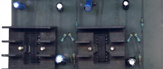
All that remains is to connect a variable resistor to the input to adjust the volume, and at this point the circuit can be considered ready for use. The circuit does not require any settings. It is enough to assemble it, solder it, plug in the op-amp and enjoy life.
As mentioned above, the circuit will be assembled on a dual op-amp, therefore, for greater convenience, the legs of the op-amp were marked on the diagram.
It is highly advisable to add 0.1 microfarad capacitors directly from the legs of the operational amplifier to ground.
Amplifier power
Power quality is very important for sound. This circuit is designed for bipolar supply voltage. This saves us from having to add unnecessary details to the sound path, and is overall better for the sound.
Today there are op amps operating from ±1.5V, but most opamps operate with a bipolar supply voltage from ±3V to ±18V. The optimal voltage is ±12V or ±15V, which is within the power supply limits of most op-amps.
The exact values of the maximum supply voltage should be found in the documentation for specific microcircuits.
To power the amplifier, it is recommended to assemble a bipolar transformer power supply. To smooth the voltage after the diode bridge, it will be sufficient to install two capacitors with a capacity of 10 μF and 100 - 470 μF.
Voltage stabilization is conveniently implemented on 7812 and 7912 chips.
To ensure good stabilization, it is necessary that the input voltage be at least 2.5-3 volts higher than the stabilization voltage.
INTRODUCTION.
I always wanted to have a more or less serious UMZCH, but in the list of life priorities it always fell to the bottom.
An alternative option was to assemble the device yourself, but I was deterred by the lack of skills to work properly with a soldering iron and the need to make a beautiful case, which I had absolutely no confidence in. The impetus for action for me was a whole series of articles “Complete amplifier on microcircuits” by Vladimir Mosyagin (MVV) in the Journal of Practical Electronics “Datagor” (link) [Complete amplifier on microcircuits. Part 1. Audio power amplifier on TDA2006, TDA2030, TDA2040, TDA2050, LM1875 I actually read a lot of articles for beginners on the basics of building ULFs, power supplies, switching, and manufacturing printed circuit boards. Then I went to Igor Rogov’s resource (Audiokiller) (link) and also read his book “Design of power supplies for audio amplifiers”
After reading everything in different sources, I realized that not everything is so scary and quite doable. Perhaps not everything will work out the first time, but still, something worthwhile should come out.
The following requirements were formulated for the final device: - presence of amplification channels for stereo speakers (SOLO-3 for now) and a separate subwoofer; — the ability to connect external signal sources, as well as the use of a permanent built-in source in the form of a Raspberry Pi, the ability to conveniently switch between sources; — expanded multimedia capabilities, connecting to TV via HDMI, watching video from a home server; — compact, laconic, pleasing to the eye device body;
Component quality
Capacitor C1 must be non-polar. Better polypropylene or film. It is better to use ceramic capacitor C2. The accuracy of capacitors is not so important, but it is better to use an accuracy of at least 5%. Resistors should preferably have an accuracy of no worse than 1%
Good microcircuits are not cheap. For example, for two original OPA2604 , which were offered in the original scheme, you will have to pay about $23.
But it is not at all necessary to immediately purchase the most expensive. To begin with, you can supply something from the assortment of the nearest radio parts store, and gradually replace them with higher quality components. The board will work on any parts.
Prices for operational amplifiers vary widely and more expensive does not always mean better sound. To begin with, you can install something inexpensive and accessible, for example, the beloved NE5532 ($0.3). It is highly desirable that it be made by Phillips.
Subsequently, you can play with replacing the op-amp as much as you want. If we consider op-amps of a higher class, then OPA2134, OPA2132, OPA2406, AD8066, AD823, AD8397… have proven themselves well for sound.
Do not order the cheapest microcircuits from AliExpress and other Chinese stores. There are a lot of fake chips out there. They will work as expected, but it may not be the OPA2134 you ordered, but a rather cheap TL061 labeled OPA2134...
But I managed to find a store that sells truly original microcircuits. And in general it has very high quality audio components. Including the top ones. I highly recommend this store.